This chapter links to the course’s interactive demos and uses MathJax for its formulas. Read it through the course website (or download the file and open it in a browser); a Canvas inline preview will reach neither the demos nor the math. All chapters.
Affine Transformations over Homogeneous Coordinates
Homogeneous coordinates were introduced by August Ferdinand Möbius in 1827, in Der barycentrische Calcul; Lawrence Roberts brought them to 3D computer graphics in his 1963 MIT thesis. Möbius, 1827; Roberts, Machine Perception of Three-Dimensional Solids, MIT, 1963
To place a model in a scene you translate, rotate, scale and sometimes shear it, in some order, and then undo those operations for picking and for cameras. All of these are one kind of map, an affine map: a linear part and a shift, and one extra coordinate, \(w\), turns the whole family into a single matrix multiplication. The chapter starts with that coordinate and the reasons graphics uses it, names the family and what it preserves, and derives from two block formulas what the pipeline needs: why composition order matters, the inverse, a matrix read as a coordinate frame and read backward as a change of coordinates, the TRS form engines store and the shear it cannot hold, the rule for transforming normals, pivots and conjugation, and the boundary of the family, where the perspective matrix leaves it. It also settles which way round the sixteen numbers are stored. The Appendix holds the conditioning of the inverse, the polar decomposition and the transformation of planes. The pictures are two-dimensional wherever the idea allows, and every number is computed by the course’s own transform library.
- Homogeneous coordinates, and why graphics uses them
- Affine maps and what they preserve
- Homogeneous coordinates: the lift
- Composition, and why order matters
- The inverse
- A matrix is a frame; object and world space
- TRS, and the shear it cannot store
- Normals transform by the inverse transpose
- Pivots and conjugation
- Where affine ends
- In code
- Exercises
0 · Homogeneous coordinates, and why graphics uses them
Homogeneous coordinates add one number, \(w\), to every point: the 2D point \((x, y)\) is written \((x, y, 1)\) and the 3D point \((x, y, z)\) is written \((x, y, z, 1)\). Any nonzero multiple names the same point, so \((x, y, w)\) is the point \((x/w,\, y/w)\). Seen one dimension up, a homogeneous point is a whole ray through the origin, and the ordinary point is where that ray crosses \(w = 1\), found by dividing by \(w\).
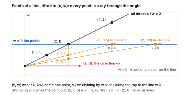
Graphics uses this representation for four reasons.
- One matrix for every placement. Rotation, scale and shear are matrix products, but translation is an addition. With \(w\) all four become one \(3\times3\) product in 2D or one \(4\times4\) product in 3D (Section 2), and a chain of placements multiplies down to one matrix (Section 3).
- Perspective. A matrix can write a point’s depth into \(w\); dividing \(x, y, z\) by \(w\) afterward makes distant things smaller. That is the perspective projection of the viewing chapter, and Section 9 is where it leaves the affine family.
- Points at infinity. \((x, y, z, 0)\) never reaches \(w = 1\): it is a direction, which no translation moves (Sections 1.2 and 2). A light placed there is a directional light, such as the sun.
- One data type from file to shader. Shading languages make the 4-vector
(
vec4in GLSL, the OpenGL Shading Language;float4in HLSL, the High-Level Shading Language) and the \(4\times4\) product built-in types, so vertices, matrices and shader math share one representation. The first programmable vertex processors (DirectX 8 vertex shaders, 2000, in hardware on the GeForce 3 in 2001) computed on four-component registers. NVIDIA’s G80 (2006) and AMD’s GCN (2012) moved to scalar instructions per thread, so on a current GPU (graphics processing unit) avec4operation is four scalar ones; the four-wide representation stayed.
_WorldSpaceLightPos0 as (direction, 0) or (position, 1).
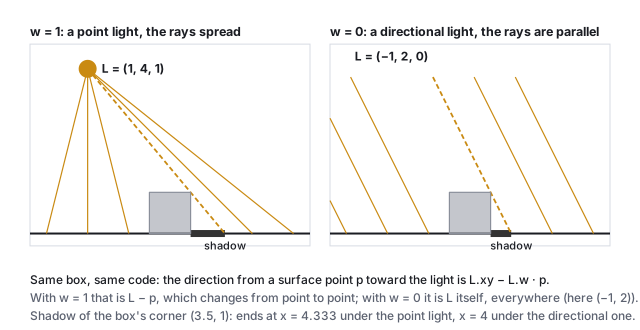
1 · Affine maps and what they preserve
| map | \(A\) | \(\mathbf{t}\) |
|---|---|---|
| translation by \(\mathbf{t}\) | \(I\) | \(\mathbf{t}\) |
| rotation \(R\) about the origin | \(R\) | \(0\) |
| scale by \((s_x, s_y, s_z)\) | \(\mathrm{diag}(s_x, s_y, s_z)\) | \(0\) |
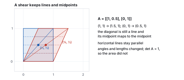
| shear \(x' = x + k\,y\) | \(\begin{pmatrix} 1 & k & 0 \\ 0 & 1 & 0 \\ 0 & 0 & 1\end{pmatrix}\) | \(0\) |
| any composition of these | a product of the \(A\)’s | some vector (Section 3) |
1.1 The determinant: volume and handedness
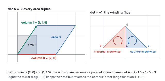
\(\det A\) is the factor by which \(A\) scales volume (the scalar triple product of its columns, the vectors chapter, Section 3.2), and its sign says whether handedness flipped. Computed by the library:
| \(A\) | \(\det A\) | meaning |
|---|---|---|
| \(\mathrm{diag}(2, 1, 1)\) | \(2\) | twice the volume |
| \(R_y(60^\circ)\) | \(1\) | a rotation keeps volume and handedness |
| \(\mathrm{diag}(-1, 1, 1)\) | \(-1\) | a mirror: same volume, right hand to left hand |
| the shear above | \(1\) | area kept, shape not |
| a zero scale | \(0\) | a dimension collapsed; no inverse |
1.2 Points move; displacements do not
\[ f(\mathbf{p}) - f(\mathbf{q}) = (A\mathbf{p} + \mathbf{t}) - (A\mathbf{q} + \mathbf{t}) = A\,(\mathbf{p} - \mathbf{q}). \]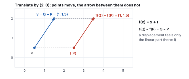
A position is a place and moves with the world; a direction has no place and must not move when the world is shifted. Section 2 makes the matrix enforce this automatically.
2 · Homogeneous coordinates: the lift
Append a \(1\) to every point, \((x, y, z)\mapsto(x, y, z, 1)\), and pack \(A\) and \(\mathbf{t}\) into one \(4\times4\) matrix:
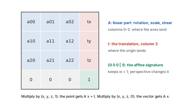
In two dimensions the same construction is a \(3\times3\): translation by \((t_x, t_y)\) is \(\begin{pmatrix} 1 & 0 & t_x \\ 0 & 1 & t_y \\ 0 & 0 & 1 \end{pmatrix}\), and \((x, y, 1)\mapsto(x + t_x,\, y + t_y,\, 1)\). In the three-dimensional \((x, y, w)\) space this matrix is linear: it fixes the origin and slides each horizontal layer by \(w\) times \(\mathbf{t}\), a shear. The floor \(w = 0\) does not move; the plane \(w = 1\), where the points live, moves by \(\mathbf{t}\). Translation, which no \(2\times2\) matrix can do, is a shear one dimension up.
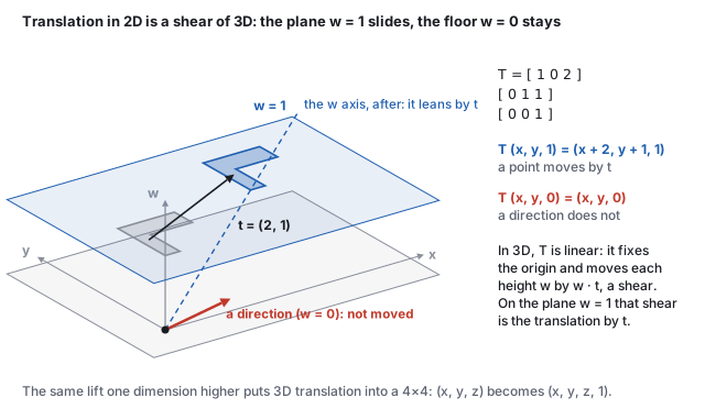
makeTRS on the plane \(z = 0\).This is the entire engineering reason for \(4\times4\) matrices in graphics: translation, rotation, scale and shear become one data type with one multiply, one inverse, and one upload to the GPU. The \(w\) arithmetic is a pleasant type check: point minus point gives \(w = 0\), a vector; point plus vector gives \(w = 1\), a point.
2.1 Sixteen numbers, two conventions
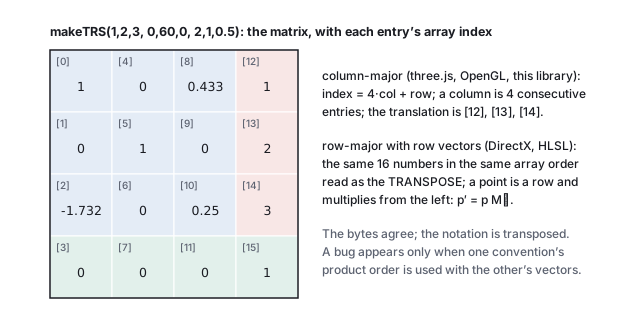
A \(4\times4\) matrix is sixteen numbers in memory, and two decisions turn them into a matrix: whether consecutive numbers run down a column or along a row (column-major or row-major storage), and whether a point is a column that the matrix multiplies from the left, \(\mathbf{p}' = M\mathbf{p}\), or a row that multiplies the matrix from the right, \(\mathbf{p}' = \mathbf{p}M\) (column-vector or row-vector convention). The mathematics is identical, since \((M\mathbf{p})^{\mathsf T} = \mathbf{p}^{\mathsf T}M^{\mathsf T}\); the bookkeeping is not.
| system | vectors | storage | “rotate then translate” is written | translation lives at |
|---|---|---|---|---|
OpenGL, three.js, this library, Unity’s Matrix4x4 | column | column-major | \(T\cdot R\) | indices 12, 13, 14 (the last column) |
| DirectX, HLSL by default, Unreal | row | row-major | \(R\cdot T\) | indices 12, 13, 14 (the last row) |
| textbooks, this text | column | as printed | \(T\cdot R\) | the last column |
invertTRS refuses such a
matrix with an explicit message rather than inverting it wrongly. Composition order errors
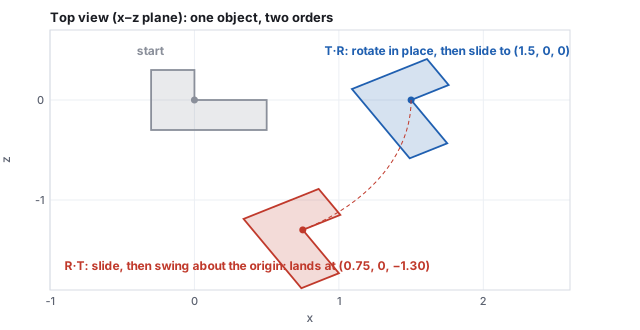
are the milder cousin: writing \(R\cdot T\) where \(T\cdot R\) was meant puts the object on an
arc instead of at its position, which Section 3 shows.
3 · Composition, and why order matters
Do \(f(\mathbf{x}) = A\mathbf{x} + \mathbf{t}\), then \(g(\mathbf{x}) = B\mathbf{x} + \mathbf{s}\):
\[ g(f(\mathbf{x})) = B(A\mathbf{x} + \mathbf{t}) + \mathbf{s} = (BA)\,\mathbf{x} + (B\mathbf{t} + \mathbf{s}). \]On column vectors, the matrix nearest the vector acts first, so a product \(B\cdot A\) means “\(A\) first, then \(B\)” and is read right to left, the same convention as the quaternion product in the rotation chapter. A chain of placements, an arm on a base on a table, is a product of several such matrices, and the scene-graph chapter is this formula applied down a tree.
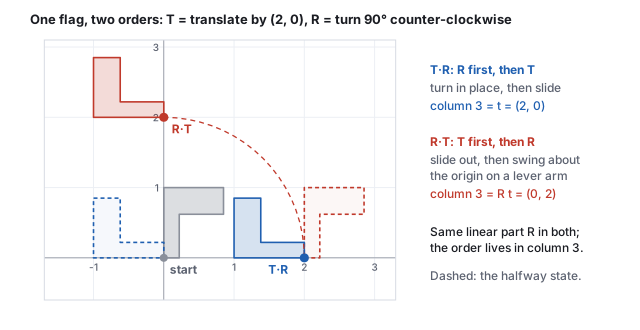
| \(T\cdot R\) | second map \(T\): \(B = I\), \(\mathbf{s} = \mathbf{t}\); first map \(R\): \(A = R\), translation \(0\). Linear part \(R\); translation \(I\cdot 0 + \mathbf{t} = (1.5, 0, 0)\). |
| \(R\cdot T\) | second map \(R\): \(B = R\), \(\mathbf{s} = 0\); first map \(T\): \(A = I\), translation \(\mathbf{t}\). Linear part \(R\); translation \(R\,\mathbf{t} = (1.5\cos60^\circ, 0, -1.5\sin60^\circ) = (0.75, 0, -1.299)\). |
matMul(makeTRS(…), makeTRS(…)), and they are what the demo’s panels print.
4 · The inverse
Solve \(\mathbf{y} = A\mathbf{x} + \mathbf{t}\) for \(\mathbf{x}\): \(\mathbf{x} = A^{-1}\mathbf{y} - A^{-1}\mathbf{t}\).
invertTRS assembles.
The reversal rule for products is the socks-then-shoes rule: to undo, take the shoes off first. The two uses that matter most: bringing a world point into an object’s own frame for a hit test (Section 5), and the view matrix, which is the inverse of the camera’s placement (the viewing chapter).
invertTRS returns exactly this matrix, and
\(M\cdot M^{-1}\) evaluates to the identity in every entry.
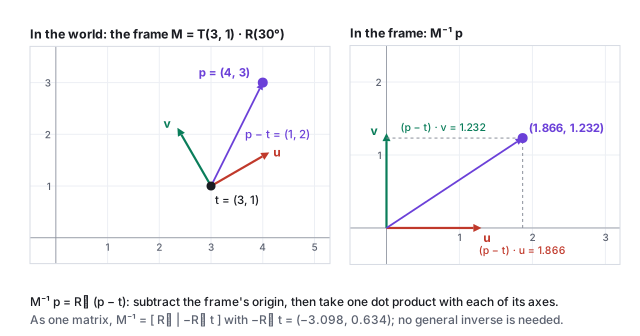
The rigid inverse has a picture. \(M^{-1}\mathbf{p} = R^{\mathsf T}(\mathbf{p} - \mathbf{t})\): subtract the frame’s origin, then measure along the frame’s axes, one dot product each, because the rows of \(R^{\mathsf T}\) are the columns of \(R\), the frame’s axes.
5 · A matrix is a frame; object and world space
Feed the matrix the basis vectors and the origin, in homogeneous form:
\[ \begin{aligned} M\,(1,0,0,0)^{\mathsf T} &= \text{column 0}, & M\,(0,1,0,0)^{\mathsf T} &= \text{column 1}, \\ M\,(0,0,1,0)^{\mathsf T} &= \text{column 2}, & M\,(0,0,0,1)^{\mathsf T} &= \text{column 3}. \end{aligned} \]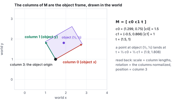
Every object has its own frame, the one its mesh was authored in (a cube’s corners at
\(\pm\tfrac12\), forever). The model matrix \(M\) is the bridge:
\(\mathbf{p}_{\text{world}} = M\,\mathbf{p}_{\text{object}}\) places the mesh without touching its
vertices, and \(\mathbf{p}_{\text{object}} = M^{-1}\mathbf{p}_{\text{world}}\) brings a world point (a
mouse ray’s hit, another object’s position) into the object’s frame for tests like
“is this point inside me”. In Unity, transform.localPosition lives in the
parent’s frame and transform.position in the world; the difference is exactly the
parent chain, which the scene-graph chapter composes
and inverts.
5.1 Active and passive: one matrix, two readings
The same matrix answers two questions. Read actively, \(M\) moves the object: the cube’s corner at object \((\tfrac12, \tfrac12)\) is carried to world \((1.9, 1.808)\). Read passively, \(M\) changes coordinates: the world point \((1.9, 1.808)\), which never moved, has coordinates \((\tfrac12, \tfrac12)\) when measured along the object’s axes from the object’s origin, and \(M^{-1}\) is the map that measures. When the columns are orthonormal the passive reading is the dot-product recipe of the vectors chapter, Section 1.1; when they are not, it is a linear solve, which the inverse packages.
5.2 One throw, one chain
A placement is usually a product of several frames, each one simple in its own coordinates. A spiral pass, from the ball’s vertices to a pixel:
\[ \mathbf{p}_{\text{clip}} = P\,V\,F\,H\,T(t)\,A(t)\,W(t)\,S(t)\,\mathbf{p}_{\text{mesh}}. \]Read from the right, each factor maps one frame into the next:
| Link | Matrix | From → to |
|---|---|---|
| \(S(t)\), spin | \(R_z(\varphi)\), \(\varphi = 2\pi\cdot\tfrac{\text{rpm}}{60}\cdot t\) | object → spin axis |
| \(W(t)\), wobble | \(R_z(\psi)\,R_x(\beta)\,R_z(-\psi)\), \(\psi = 2\pi f t\) | spin axis → velocity |
| \(A(t)\), aim | \(R_x(-\theta)\), \(\theta = \operatorname{atan2}(v_y, v_z)\) | velocity → flight |
| \(T(t)\), flight | translation by \((0,\; v\sin\alpha\,t - \tfrac12 g t^2,\; v\cos\alpha\,t)\) | flight → throw |
| \(H\), set-up | \(T(\mathbf{s})\,R_y(h)\): release point \(\mathbf{s}\), heading \(h\) | throw → field |
| \(F\), field | \(R_y(\gamma)\,T(-25, 0, -55)\) | field → world |
| \(V\), view | \((F\,C)^{-1}\), \(C\) the camera’s placement in the field | world → camera |
| \(P\), projection | a perspective map (the viewing chapter) | camera → clip |
The ball is modeled with its long axis on \(+z\) and its laces on \(+y\), so the spin is a rotation about its own \(z\). \(W\) is the pivot sandwich of Section 8: the tilt \(R_x(\beta)\) done in a frame turned by \(\psi\) about \(z\), so the nose circles the direction of flight on a cone of half-angle \(\beta\), the wobble of a real spiral. \(A\) turns \(+z\) onto the velocity; a positive turn about \(x\) carries \(+z\) toward \(-y\), hence the minus sign. \(T\) is a pure translation, so the flight frame keeps the throw frame’s axes and the path lies in the throw frame’s \(yz\) plane. \(H\) and \(F\) are built once, from the throw’s parameters. Every partial product is a frame placement: \(F H\) is the throw frame in the world, \(F H\,T(t)\) the frame at the ball’s center, and column 3 of each is where that frame’s origin is.
A chain can also change its root. In the demo a cart carrying an open bowl drives to where the ball comes
down and catches it at \(t_c\). From then on the ball is the cart’s child, and its placement must not
jump at the switch, so its new local matrix is its old placement measured in the cart’s frame,
\(L = K(t_c)^{-1}\,H\,T\,A\,W\,S\,(t_c)\), and afterwards it is \(F\,K(t)\,L\): the cart’s
placement \(K(t)\) times a constant. That is what Unity’s SetParent(cart, true)
(“world position stays”) computes, and what three.js’s Object3D.attach does.
lib/assets/models/football/.
6 · TRS, and the shear it cannot store
Any invertible \(A\) factors as a rotation times a symmetric stretch, \(A = R\,P\) (the polar decomposition, Appendix A.2). Engines store the special case in which the stretch is axis-aligned:
\[ \begin{gathered} M = T\cdot R\cdot S, \\ \text{columns 0 to 2} = \text{the rotated axes, each scaled by its factor}, \qquad \text{column 3} = \mathbf{t}. \end{gathered} \]makeTRS(1,2,3, 0,60,0, 2,1,0.5) is
\[
M = \begin{pmatrix} 1 & 0 & 0.433 & 1 \\ 0 & 1 & 0 & 2 \\ -1.732 & 0 & 0.25 & 3 \\ 0 & 0 & 0 & 1 \end{pmatrix}.
\]
Column lengths: \(\|(1, 0, -1.732)\| = 2\), \(\|(0,1,0)\| = 1\), \(\|(0.433, 0, 0.25)\| = 0.5\): the
scale \((2, 1, 0.5)\). Normalize the columns: \((0.5, 0, -0.866)\), \((0,1,0)\), \((0.866, 0, 0.5)\),
the columns of \(R_y(60^\circ)\). Column 3 is \((1, 2, 3)\). This read-back is the first step of
invertTRS, and it silently assumes the normalized columns are orthonormal.
An affine map has twelve degrees of freedom (nine in \(A\), three in \(\mathbf{t}\)). A
Transform stores nine: position, a rotation (three degrees of freedom, as a quaternion), and
three scale factors. The missing three are shear: \(T\cdot R\cdot S\) cannot
represent a sheared object. This is not academic. A child rotated \(45^\circ\) under a parent
scaled non-uniformly is sheared in world space; Unity’s Transform cannot hold that
matrix, and its lossyScale property is the honest admission that the world-space scale
it reports is an approximation.
6.1 What the read-back does to a shear
The stretch need not come from a shear matrix. Scaling by 2 along the diagonal \((1, 1, 0)/\sqrt2\), the conjugation \(R_z(45^\circ)\,\mathrm{diag}(2, 1, 1)\,R_z(-45^\circ)\) of Section 8, is a symmetric matrix with no rotation at all, and TRS cannot hold it either:
invertTRS makes of it)
\(M = \begin{pmatrix} 1.5 & 0.5 & 0 \\ 0.5 & 1.5 & 0 \\ 0 & 0 & 1 \end{pmatrix}\): \(M(1, 1, 0) = (2, 2, 0)\)
(stretched twice along the diagonal) and \(M(1, -1, 0) = (1, -1, 0)\) (unchanged across it),
\(\det M = 2\). Its first two columns have length \(1.581\) each and dot product \(1.5\), an angle
of \(53.1^\circ\), not \(90^\circ\). The TRS read-back reports scale \((1.581, 1.581, 1)\) and a
“rotation” whose columns are not orthogonal, and invertTRS, which trusts
the read-back, returns a matrix whose first column is \((0.6, 0.2, 0)\) where the true inverse
has \((0.75, -0.25, 0)\); \(M\) times that answer has \(0.6\) in an entry that should be 0.
The shear of Appendix A.2 fails the same way: its columns have lengths \(1\) and \(1.118\) and meet at
\(63.4^\circ\).
7 · Normals transform by the inverse transpose
A tangent direction \(\mathbf{d}\) is a difference of points and transforms by \(A\). A normal is defined by being perpendicular to tangents, and \(A\mathbf{n}\) is not, in general, perpendicular to \(A\mathbf{d}\). What is: \(A^{-\mathsf T}\mathbf{n}\), because \((A\mathbf{d})\cdot(A^{-\mathsf T}\mathbf{n}) = \mathbf{d}^{\mathsf T}A^{\mathsf T}A^{-\mathsf T}\mathbf{n} = \mathbf{d}\cdot\mathbf{n} = 0\).
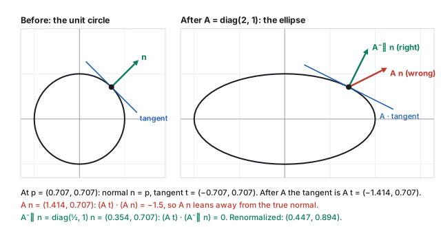
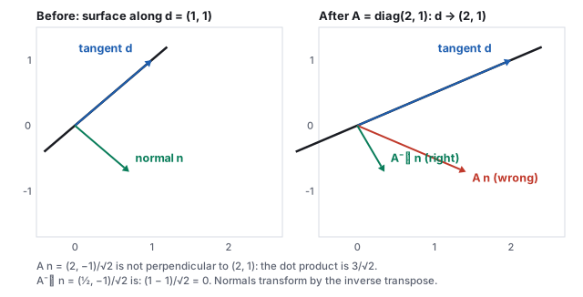
| tangent after | \(A\mathbf{d} = (2, 1, 0)\) |
| naive | \(A\mathbf{n} = (1.414, -0.707, 0)\); \((2,1,0)\cdot(1.414, -0.707, 0) = 2.828 - 0.707 = 2.121 \ne 0\) |
| inverse transpose | \(A^{-\mathsf T} = \mathrm{diag}(\tfrac12, 1, 1)\); \(A^{-\mathsf T}\mathbf{n} = (0.354, -0.707, 0)\); \((2,1,0)\cdot(0.354, -0.707, 0) = 0.707 - 0.707 = 0\) |
8 · Pivots and conjugation
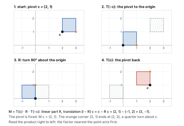
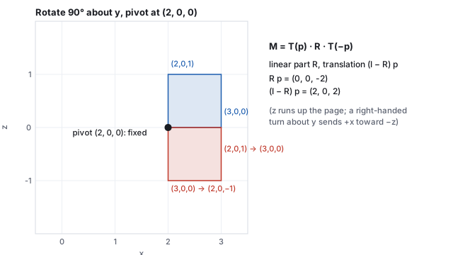
\(R\) spins about the origin. To spin about a point \(\mathbf{p}\), bring \(\mathbf{p}\) to the origin, rotate, and send it back, and apply the block product of Section 3:
\[ M = T(\mathbf{p})\cdot R\cdot T(-\mathbf{p}) \;=\; \begin{pmatrix} R & \mathbf{p} - R\mathbf{p} \\ \mathbf{0}^{\mathsf T} & 1 \end{pmatrix} = \begin{pmatrix} R & (I - R)\,\mathbf{p} \\ \mathbf{0}^{\mathsf T} & 1 \end{pmatrix}. \]\(\mathbf{p}\) is the fixed point: \(T(-\mathbf{p})\) sends it to the origin, \(R\) leaves the origin, \(T(\mathbf{p})\) returns it. Swap \(R\) for \(S\) to scale about a point. Every off-center rotation, joint articulation and scale-about-a-corner is this conjugation, and the translation column \((I - R)\mathbf{p}\) is a number nobody would enter by hand, which is why the sandwich is built rather than typed.
9 · Where affine ends
Homogeneous coordinates are defined only up to scale: \((x, y, z, w)\) and \((\lambda x, \lambda y, \lambda z, \lambda w)\) name the same point, \((x/w, y/w, z/w)\). An affine matrix never changes \(w\), so the divide is invisible. A general \(4\times4\) whose last row is not \((0,0,0,1)\) does change it, and the map it defines after the divide is projective: lines still go to lines, but parallel lines can meet and ratios along a line are not kept.
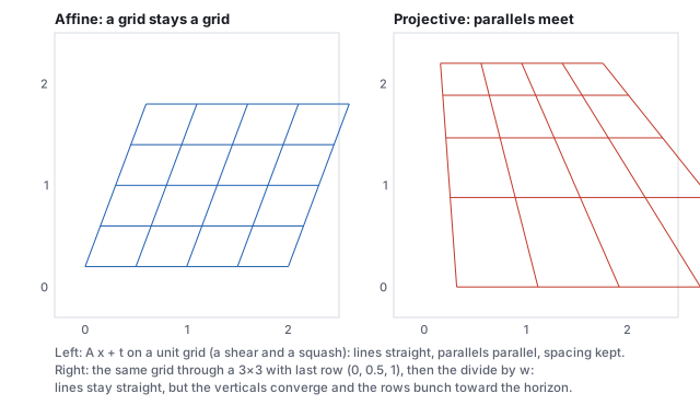
| in | \(w\) | out |
|---|---|---|
| \((1, 0)\) | 1 | \((1, 0)\) |
| \((1, 1)\) | 1.5 | \((0.667, 0.667)\) |
| \((1, 2)\) | 2 | \((0.5, 1)\) |
Three consequences. The perspective projection of the
viewing chapter deliberately writes \(-z\) into \(w\), so that dividing by \(w\) divides by
depth and distant things shrink; it is the one non-affine matrix in the pipeline, and the
divide by \(w\) is its signature. A vector with \(w = 0\) is, in this language, a point at
infinity: a direction is where parallel lines meet, which is why directions never move
under translation. And the library’s invertTRS refuses a matrix whose last row is
not \((0,0,0,1)\), because the block inverse of Section 4 only holds inside the affine family;
the interaction chapter inverts the full projective
matrix by elimination to send a mouse position back into the world.
10 · In code
css551/ directory. Matrices print as their 16-element
column-major arrays: four numbers per column, translation last.
- The TRS matrix of Section 6 and its storage (compare with the figure of Section 2.1):
node -e "import('./lib/core/xform.js').then(x=>{console.log(x.makeTRS(1,2,3,0,60,0,2,1,0.5).map(v=>+v.toFixed(3)));})" [ 1, 0, -1.732, 0, 0, 1, 0, 0, 0.433, 0, 0.25, 0, 1, 2, 3, 1 ] - The translation columns of \(T\cdot R\) and \(R\cdot T\) (Section 3):
node -e "import('./lib/core/xform.js').then(x=>{const T=x.makeTRS(1.5,0,0,0,0,0,1,1,1),R=x.makeTRS(0,0,0,0,60,0,1,1,1);console.log(x.matMul(T,R).slice(12,15).map(v=>+v.toFixed(3)), x.matMul(R,T).slice(12,15).map(v=>+v.toFixed(3)));})" [ 1.5, 0, 0 ] [ 0.75, 0, -1.299 ] - A round trip through a TRS matrix and its inverse (in double precision; Appendix A.1 measures the float32 version):
node -e "import('./lib/core/xform.js').then(x=>{const M=x.makeTRS(1,2,3,30,60,10,2,1,0.5);const p=x.applyMat4(M,[1,1,1]);console.log(x.applyMat4(x.invertTRS(M),p.slice(0,3)).slice(0,3).map(v=>+v.toFixed(6)));})" [ 1, 1, 1 ] - The refusal on a projective matrix (Section 9):
node -e "import('./lib/core/xform.js').then(x=>{try{x.invertTRS(x.perspective(45,1.78,1,8))}catch(e){console.log(e.message)}})" invertTRS: bottom row must be (0,0,0,1) ... Got a perspective/shear-shaped bottom row. - The silent failure on an oblique scale (Section 6.1): the call succeeds and the first column of its answer is wrong:
node -e "import('./lib/core/xform.js').then(x=>{const Rd=x.axisAngleMatrix(0,0,1,45),S=x.makeTRS(0,0,0,0,0,0,2,1,1);const M=x.matMul(x.matMul(Rd,S),x.invertTRS(Rd));console.log(x.invertTRS(M).slice(0,3).map(v=>+v.toFixed(3)));})" [ 0.6, 0.2, 0 ] - In the order demo, set the rotation to \(180^\circ\) with the translation at \(1.5\): the \(R\cdot T\) cube lands at \(x = -1.5\), the \(T\cdot R\) cube at \(+1.5\), the widest the two orders can disagree.
11 · Exercises
Solution
\(T\cdot S\): \(B = I\), so the column is \(I\cdot0 + (1,0,0) = (1,0,0)\); the origin lands at \((1,0,0)\). \(S\cdot T\): \(B = 2I\), column \(2I\cdot(1,0,0) + 0 = (2, 0, 0)\); the origin lands at \((2,0,0)\). Scaling after translating scales the translation too.Solution
\(R_z(90^\circ)\) has columns \((0,1,0), (-1,0,0), (0,0,1)\); \(R^{\mathsf T}\mathbf{t} = \big((0,1,0)\cdot(0,3,0),\; (-1,0,0)\cdot(0,3,0),\; 0\big) = (3, 0, 0)\), so the inverse has linear part \(R^{\mathsf T}\) and translation \((-3, 0, 0)\). Forward: \(M(1,0,0) = R(1,0,0) + \mathbf{t} = (0,1,0) + (0,3,0) = (0,4,0)\). Back: \(R^{\mathsf T}(0,4,0) + (-3,0,0) = (4, 0, 0) + (-3, 0, 0) = (1, 0, 0)\).Solution
Position \((5,5,5)\); scale \((2, 3, 1)\) from the column lengths; normalized columns \((0,1,0), (-1,0,0), (0,0,1)\) are \(R_z(90^\circ)\). Determinant of the normalized part is \(+1\) (a rotation), so right-handed; with the scale, \(\det = 6 > 0\).Solution
\(A^{-\mathsf T} = \mathrm{diag}(1, 1, \tfrac13)\): \((0, 0.707, 0.236)\), renormalized \((0, 0.949, 0.316)\). Stretching along \(z\) makes the surface flatter, so its normal tilts toward \(y\), away from the stretch; the naive \(A\mathbf{n} = (0, 0.707, 2.121)\) tilts the wrong way.Solution
Linear part \(2I\); translation \((I - 2I)\mathbf{p} = -\mathbf{p} = (-1, -1, 0)\). \(M(1,1,0) = (2,2,0) + (-1,-1,0) = (1,1,0)\), fixed. \(M(2,1,0) = (4,2,0) + (-1,-1,0) = (3,1,0)\): the point one unit right of the pivot is now two units right.Solution
\(w = 1 + 3 = 4\): \((0.25, 1.5)\). As \(y\to\infty\), \(x/(1 + 0.5y)\to0\) and \(y/(1 + 0.5y)\to 2\): the line approaches \((0, 2)\), the vanishing point shared by every vertical line.Solution
Index \(4\cdot0 + 2 = 2\), value \(-1.732\) (the \(-\sin 60^\circ\) of \(R_y\), times the scale 2). The row-vector system stores the transpose row-major, which is the same sixteen numbers in the same order, so \(t_y\) is again at index 13; only the reading changes.Solution
\((1.5, 1)\) is the frame’s origin, column 3: object \((0, 0)\). \((2.799, 1.75) - (1.5, 1) = (1.299, 0.75) = \mathbf{c}_0\): object \((1, 0)\), the far end of the object’s stretched \(x\) axis. Recognizing a column saves the solve; for any other point the inverse of the worked example does it.axisAngleMatrix, makeTRS and matMul, print the dot product of its first two columns, and explain the number.
Solution
node -e "import('./lib/core/xform.js').then(x=>{const R=x.axisAngleMatrix(0,0,1,30),S=x.makeTRS(0,0,0,0,0,0,3,1,1);const M=x.matMul(x.matMul(R,S),x.invertTRS(R));console.log(x.dot([M[0],M[1],M[2]],[M[4],M[5],M[6]]).toFixed(4));})" prints 3.4641. The matrix is symmetric, \(\begin{pmatrix} 2.5 & 0.866 \\ 0.866 & 1.5 \end{pmatrix}\) in its \(xy\) block, and \(2.5\cdot0.866 + 0.866\cdot1.5 = 3.464\) is far from the 0 of orthogonal columns: a stretch along a tilted axis is not a TRS matrix, and the read-back would report a scale of \(2.65\) and \(1.73\) with a bogus rotation.
Solution
\(V_{\text{ball}} = (F\,C_{\text{ball}})^{-1} = K^{-1}A^{-1}T^{-1}H^{-1}F^{-1}\) and \(V_{\text{spin}} = K^{-1}S^{-1}W^{-1}A^{-1}T^{-1}H^{-1}F^{-1}\): the inverse of a product is the product of the inverses in reverse order. The spin camera’s view matrix carries the extra \(S(t)^{-1} = R_z(-\varphi)\), a turn about the ball’s long axis, which is nearly the camera’s line of sight, so the world rolls by \(-\varphi\): ten turns a second at 600 rpm. The ball, a child of the same frame, holds still in that picture. A camera inherits every link between it and the root; mount it above the links whose motion the picture should not show.Appendix
A.1 Conditioning: how much precision the inverse costs
An inverse exists whenever \(\det A \ne 0\), but existing and being computable in single precision are different things. The condition number \(\kappa(A)\), the ratio of the largest to the smallest stretch \(A\) applies to any direction, bounds how much a relative error in the input grows in the output: a round trip \(\mathbf{x}\to M\mathbf{x}\to M^{-1}(M\mathbf{x})\) in arithmetic with relative precision \(\varepsilon\) returns \(\mathbf{x}\) only to about \(\kappa\,\varepsilon\). For a rotation \(\kappa = 1\); for \(\mathrm{diag}(s, 1, 1)\), \(\kappa = s\).
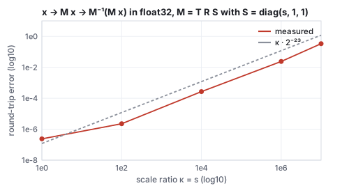
| scale ratio \(s = \kappa\) | 1 | \(10^2\) | \(10^4\) | \(10^6\) | \(10^7\) |
|---|---|---|---|---|---|
| round-trip error of \((1,1,1)\) | \(2.4\times10^{-7}\) | \(2.3\times10^{-6}\) | \(2.7\times10^{-4}\) | \(2.4\times10^{-2}\) | \(0.34\) |
| \(\kappa\cdot2^{-23}\) | \(1.2\times10^{-7}\) | \(1.2\times10^{-5}\) | \(1.2\times10^{-3}\) | \(0.12\) | \(1.2\) |
A.2 The polar decomposition
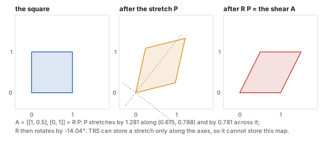
A.3 Planes
A plane is a normal and an offset, and the two travel together. Write the plane \(\hat{\mathbf{n}}\cdot P = D\) of the vectors chapter as the homogeneous row \(\boldsymbol\pi = (n_x, n_y, n_z, -D)\), so that a point is on the plane exactly when \(\boldsymbol\pi\cdot(x, y, z, 1) = 0\). If points move by \(M\), the plane through their images must satisfy \(\boldsymbol\pi'\cdot(M\tilde{\mathbf{p}}) = 0\) whenever \(\boldsymbol\pi\cdot\tilde{\mathbf{p}} = 0\), which holds for \(\boldsymbol\pi' = M^{-\mathsf T}\boldsymbol\pi\): the full \(4\times4\) inverse transpose, which moves the offset as well as tilting the normal. Renormalize the first three components afterward and \(-\boldsymbol\pi'_3\) is the new \(D\).
makeTRS(1,2,3, 0,60,0, 2,1,0.5).
\(M^{-\mathsf T}\boldsymbol\pi = (1.238, 0.667, 0.522, -4.472)\), normalized on its first three components to
\((0.825, 0.444, 0.348, -2.981)\): the new normal is \((0.825, 0.444, 0.348)\) and the new offset
\(D' = 2.981\). Check on two points known to be on the old plane, \(Q = (1, 0, 0)\) and the foot
\((3.444, -0.111, -1.111)\): their images \(M Q = (2, 2, 1.268)\) and \((3.963, 1.889, -3.243)\) both
satisfy \(\hat{\mathbf{n}}'\cdot P - D' = 0\) to six decimals. The naive normal \(A\hat{\mathbf{n}}\),
normalized to \((0.622, 0.667, -0.411)\), fails: the two image points differ by \(3.0\) in
their “signed distance” from a plane that should contain both. Clipping planes,
mirrors and shadow-caster planes all move this way.