This chapter links to the course’s interactive demos and uses MathJax for its formulas. Read it through the course website (or download the file and open it in a browser); a Canvas inline preview will reach neither the demos nor the math. All chapters.
Viewing: the Camera, the View Matrix, and Projection
Filippo Brunelleschi demonstrated linear perspective in Florence around 1415, with a painted panel of the Baptistery viewed through a hole and a mirror. Antonio Manetti, Life of Brunelleschi, 1480s
Placing objects in a world produces nothing visible until someone says where the viewer stands and which way they look. Two matrices turn a placed world into a flat image: the view matrix, which re-expresses the world in the camera’s own coordinate frame, and the projection matrix, which flattens depth by dividing by it. This chapter builds both from the vectors and affine maps of the earlier chapters: three cross products for the camera’s axes, the rigid inverse for the view matrix, similar triangles for the perspective divide, and a \(4\times4\) whose last row is the one non-affine row in the pipeline. It then goes where a renderer has to go next: what a field of view means in a photographer’s millimeters, what a 24-bit or a floating-point depth buffer can and cannot tell apart and why reversing the depth range helps by a factor of a thousand, how the six planes of the frustum fall out of the projection matrix and cull a box in six dot products, how an asymmetric frustum serves a stereo display, and what a real lens adds that the pinhole omits. Every matrix is the course library’s own, on the demos’ own cameras, and one vertex is followed through the whole chain to the pixel and the depth value it lands on.
- The camera is a frame
- The view matrix
- Perspective: divide by depth
- Field of view, focal length, aspect
- The projection matrix, entry by entry
- Depth, near and far
- What a depth buffer can resolve
- The full chain, for one vertex
- The frustum’s planes, and culling
- Off-axis frusta
- Orthographic projection
- Beyond the pinhole: the thin lens
- Moving the camera
- Hands-on
- Exercises
1 · The camera is a frame
A camera is pinned down by three inputs, the ones a photographer sets: a position \(\mathbf{eye}\), a target \(\mathbf{at}\), and a rough up direction \(\mathbf{up}\) (usually world \(+y\)). From them, three cross products build an orthonormal frame fixed to the camera:
This is the frame-from-two-vectors construction of the vectors chapter, with a purpose: it is the camera’s orientation. Why \(\mathbf{w}\) points backward: the projection of Section 3 assumes visible points have negative \(z\) in camera space, so the camera’s backward axis is its \(+z\), and using \(\mathbf{at} - \mathbf{eye}\) instead would produce a left-handed frame and flip the projection’s signs.
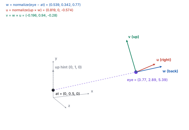
| \(\mathbf{w}\) | \(\mathbf{eye} - \mathbf{at} = (3.773, 2.394, 5.388)\), length \(7.000\); normalized \((0.539, 0.342, 0.770)\) |
| \(\mathbf{u}\) | \((0,1,0)\times\mathbf{w} = (1\cdot0.770 - 0,\; 0 - 0,\; 0 - 1\cdot0.539) = (0.770, 0, -0.539)\), normalized \((0.819, 0, -0.574)\) |
| \(\mathbf{v}\) | \(\mathbf{w}\times\mathbf{u} = (-0.196, 0.940, -0.280)\) |
2 · The view matrix
Objects live in world space; the camera renders whatever lands in its own frame. The view matrix \(V\) is the change of coordinates \(\mathbf{p}_{\text{view}} = V\,\mathbf{p}_{\text{world}}\): the same point, described in the camera’s axes, with the eye at the origin.
The rotation rows are doing real work. Replace them by the identity and keep only the
translation, and the “camera” sits in the right place but always faces world
\(-z\); aiming it at a target changes nothing. Sung’s course projects ship exactly this
broken mode, ViewMatrixWrong, as the control that proves the cross products
matter.
3 · Perspective: divide by depth
The oldest camera is a pinhole: light passes through one point onto a plane behind it, and objects farther away project smaller, which is why railroad tracks converge. Put the eye at the camera-space origin looking down \(-z\), with an image plane at distance \(d\) in front. A point at \((x, y, z)\), \(z < 0\), projects by similar triangles:
\[ \frac{y'}{d} = \frac{y}{-z} \quad\Longrightarrow\quad y' = d\,\frac{y}{-z}, \qquad x' = d\,\frac{x}{-z} . \]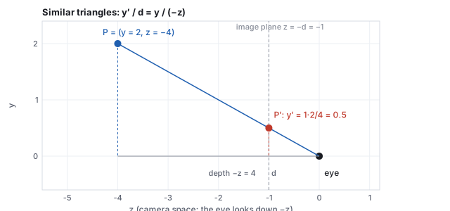
A matrix cannot divide; it can only multiply and add. The trick that makes perspective a matrix operation is the affine chapter’s boundary: write the depth into the fourth coordinate \(w'\), and let the pipeline divide every component by \(w'\) afterward. That divide, applied uniformly to every vertex, is the similar-triangles divide above. Run backward, the same fan of lines through the pinhole is the camera ray of the ray-tracing chapter and the unprojection of the interaction chapter.
4 · Field of view, focal length, aspect
The pinhole’s one free parameter is how wide a cone of the world reaches the image. Graphics states it as an angle, the vertical field of view; photography states it as a focal length in millimeters relative to a sensor of known size, and the two are one formula apart.
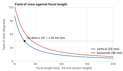
The aspect ratio also fixes the shape of the image plane: the projection scales \(x\) by \(1/a\) relative to \(y\) so that a wide framebuffer shows more world on the sides rather than a stretched one. Get \(a\) from the framebuffer’s actual pixel dimensions every time the window resizes; a projection built for \(1.78\) and drawn into a square viewport squeezes everything horizontally by a factor of \(1.78\): a square renders 1.78 times narrower than it is tall.
5 · The projection matrix, entry by entry
Every entry has a job.
- \(f\) scales \(y\) so that a point at the top edge of the field of view lands at \(y = 1\): at the edge \(y/(-z) = \tan(\text{fov}/2)\), and \(f\) times that is 1. A narrow field of view gives a large \(f\) (telephoto), a wide one a small \(f\). This \(f\) is the focal length of Section 4 in units of half the sensor height.
- \(f/a\) does the same for \(x\), divided by the aspect so a wide screen does not stretch the image.
- The \(z\) row remaps depth so that \(z = -n\) lands at \(-1\) and \(z = -f_{\!ar}\) at \(+1\) after the divide: two conditions, two unknowns (Section 6).
- The last row, \((0, 0, -1, 0)\), copies \(-z\) into \(w'\). It is the entry that makes the divide a divide by depth, and the only non-affine row in the pipeline.
6 · Depth, near and far
The \(z\) row of \(P\) is chosen so that, after the divide, \(z_{\text{ndc}} = \dfrac{A\,z + B}{-z}\) equals \(-1\) at \(z = -n\) and \(+1\) at \(z = -f_{\!ar}\). Two equations: \(-An + B = -n\) and \(-Af_{\!ar} + B = f_{\!ar}\); subtracting, \(A(n - f_{\!ar}) = f_{\!ar} + n\), so \(A = (f_{\!ar} + n)/(n - f_{\!ar})\), and substituting back \(B = 2f_{\!ar}n/(n - f_{\!ar})\). The form \(A + B/(-z)\) is forced by the divide: whatever the third row holds, dividing it by \(-z\) makes NDC depth an affine function of \(1/\text{depth}\), never of depth itself. Between the planes the map is a hyperbola, and most of the NDC range is spent close to the near plane.
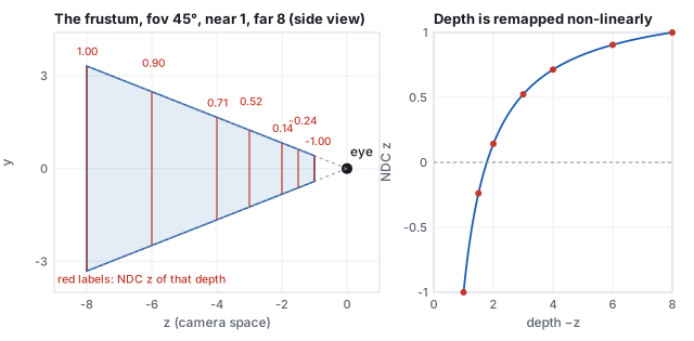
| depth \(-z\) | 1 | 1.5 | 2 | 3 | 4 | 6 | 8 |
|---|---|---|---|---|---|---|---|
| \(z_{\text{ndc}}\) | \(-1\) | \(-0.238\) | \(0.143\) | \(0.524\) | \(0.714\) | \(0.905\) | \(1\) |
Two consequences. A near plane pushed very close to zero wastes almost all of the depth buffer’s resolution on the first few centimeters, which is where distant surfaces begin to flicker through one another (“z-fighting”); the next section puts numbers on it. And the depth the rasterizer interpolates across a triangle is \(z_{\text{ndc}}\), not the view depth, which is what makes screen-space interpolation of other attributes wrong, the subject of the rasterization chapter.
7 · What a depth buffer can resolve
The depth buffer stores \(z_{\text{ndc}}\), mapped to a window depth \(z_w = (z_{\text{ndc}} + 1)/2\) in \([0, 1]\), as a 24-bit integer or a 32-bit float. The smallest difference in world depth it can tell apart at distance \(d\) is the buffer’s step at the stored value divided by the slope of the depth map there, \(\Delta d = \Delta z_w / |dz_w/dd|\), and the slope of the hyperbola falls as \(1/d^2\). The chapter’s generator evaluates this for a camera with near \(0.1\) and far \(1000\) under three formats.
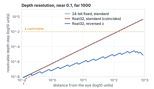
| distance | \(z_w\) | 24-bit fixed | float32 | float32, reversed |
|---|---|---|---|---|
| 0.2 | 0.50005 | \(2.4\times10^{-8}\) | \(2.4\times10^{-8}\) | \(1.2\times10^{-8}\) |
| 1 | 0.90009 | \(6.0\times10^{-7}\) | \(6.0\times10^{-7}\) | \(7.5\times10^{-8}\) |
| 10 | 0.99010 | \(6.0\times10^{-5}\) | \(6.0\times10^{-5}\) | \(9.3\times10^{-7}\) |
| 100 | 0.99910 | \(6.0\times10^{-3}\) | \(6.0\times10^{-3}\) | \(5.8\times10^{-6}\) |
| 500 | 0.99990 | \(0.149\) | \(0.149\) | \(1.8\times10^{-5}\) |
| 900 | 0.99999 | \(0.483\) | \(0.483\) | \(7.4\times10^{-6}\) |
8 · The full chain, for one vertex
Every vertex takes the same trip: object space, the model matrix \(M\) (the scene graph’s world matrix), the view matrix \(V\), the projection \(P\), the divide by \(w'\), and the viewport transform to pixels. The last step maps NDC \([-1, 1]\) to pixel columns and rows, flipping \(y\) because images count rows downward, and maps NDC depth to the window depth the buffer stores:
\[ x_{\text{px}} = \frac{x_{\text{ndc}} + 1}{2}\,W, \qquad y_{\text{px}} = \frac{1 - y_{\text{ndc}}}{2}\,H, \qquad z_w = \frac{z_{\text{ndc}} + 1}{2} . \]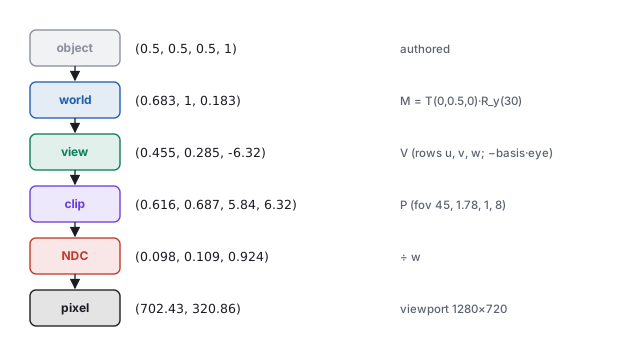
| stage | coordinates | by |
|---|---|---|
| object | \((0.5, 0.5, 0.5, 1)\) | authored |
| world | \((0.683, 1.000, 0.183)\) | \(M = T(0, 0.5, 0)\,R_y(30^\circ)\) |
| view | \((0.455, 0.285, -6.320)\) | \(V\) of Section 2; depth \(6.32\) in front of the eye |
| clip | \((0.616, 0.687, 5.840, 6.320)\) | \(P\) of Section 5; note \(w' = 6.320 = -z_{\text{view}}\) |
| NDC | \((0.098, 0.109, 0.924)\) | divide by \(w'\); inside the cube, deep in the frustum |
| pixel | \((702.7, 320.8)\), pixel \((702, 320)\), \(z_w = 0.962\) | viewport \(1280\times720\) |
9 · The frustum’s planes, and culling
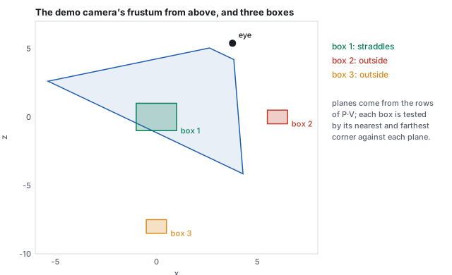
The visible region is six planes, and they can be read straight off the combined matrix \(M_{PV} = P\,V\). A point is inside the left plane exactly when its NDC \(x \ge -1\), which after the divide means clip \(x + w \ge 0\), and clip \(x\) and \(w\) are the first and fourth rows of \(M_{PV}\) dotted with the world point. So the plane is a row sum.
| box | extent | verdict | the deciding plane |
|---|---|---|---|
| 1 | \([-1,1]\times[-0.5,1.5]\times[-1,1]\) | straddles | far: p-vertex \(2.651\) inside, n-vertex \(-0.651\) outside |
| 2 | \([5.5,6.5]\times[0,1]\times[-0.5,0.5]\) | outside | right: p-vertex at \(-1.127\) |
| 3 | \([-0.5,0.5]\times[0,1]\times[-8.5,-7.5]\) | outside | far: p-vertex at \(-4.333\) |
10 · Off-axis frusta
The projection of Section 5 is symmetric: the sightline hits the center of the image. The general frustum names the near plane’s window edges \(l, r, b, t\) directly and need not be centered:
\[ P_{\text{frustum}} = \begin{pmatrix} \dfrac{2n}{r - l} & 0 & \dfrac{r + l}{r - l} & 0 \\ 0 & \dfrac{2n}{t - b} & \dfrac{t + b}{t - b} & 0 \\ 0 & 0 & \dfrac{f_{\!ar} + n}{n - f_{\!ar}} & \dfrac{2f_{\!ar}n}{n - f_{\!ar}} \\ 0 & 0 & -1 & 0 \end{pmatrix}, \]which reduces to Section 5’s \(P\) when \(l = -r\) and \(b = -t\) (the two skew entries in the third column vanish). The skew entries shift the image without turning the camera: the projection of a point moves sideways by an amount proportional to its depth, so the frustum leans while the image plane stays parallel to the sensor.
11 · Orthographic projection
Not every projection has perspective. An orthographic projection maps a rectangular box \([l, r]\times[b, t]\times[-n, -f_{\!ar}]\) to the NDC cube by scaling and offsetting each axis linearly, with \(w' = 1\) and no divide:
\[ \begin{gathered} P_{\text{ortho}} = \begin{pmatrix} \frac{2}{r - l} & 0 & 0 & -\frac{r + l}{r - l} \\ 0 & \frac{2}{t - b} & 0 & -\frac{t + b}{t - b} \\ 0 & 0 & \frac{-2}{f_{\!ar} - n} & -\frac{f_{\!ar} + n}{f_{\!ar} - n} \\ 0 & 0 & 0 & 1 \end{pmatrix}, \\[8pt] \text{for } [-4, 4]\times[-2.25, 2.25]\times[1, 8]:\quad \begin{pmatrix} 0.25 & 0 & 0 & 0 \\ 0 & 0.444 & 0 & 0 \\ 0 & 0 & -0.286 & -1.286 \\ 0 & 0 & 0 & 1 \end{pmatrix}. \end{gathered} \]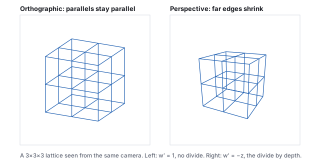
Orthographic depth is linear, so the precision argument of Section 7 does not apply and a shadow map rendered from a directional light (an orthographic camera at the sun) has uniform depth resolution across its whole range. The two projections meet in the limit: a perspective camera backed off to a great distance with a very narrow field of view is indistinguishable from an orthographic one, which is how a long lens flattens a face.
12 · Beyond the pinhole: the thin lens
A pinhole admits almost no light, so real cameras use a lens, and a lens brings only one distance into sharp focus. A point at another distance spreads into a disk on the sensor, the circle of confusion; when that disk is smaller than a pixel the point is sharp, and the range of distances for which it is sharp is the depth of field.
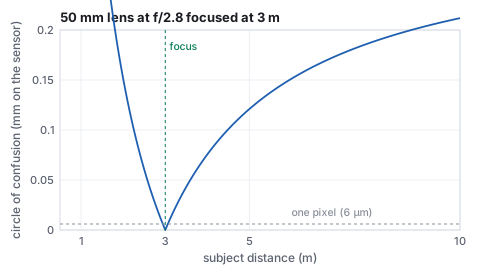
A rasterizer has no lens; it renders every depth sharp. Depth of field is added as a post-process that blurs each pixel by the circle of confusion computed from its stored depth, or in a ray tracer by starting rays from random points on the aperture disk and aiming them through the focus plane (the ray-tracing chapter’s estimator, one more dimension), which is exact and noisy. Motion blur is the same idea in time.
13 · Moving the camera
Every camera control is an edit to \(\mathbf{eye}\), \(\mathbf{at}\) or \(\mathbf{up}\), after which \(V\) is rebuilt by the three cross products. In the vocabulary of cinematography: tumble (orbit) swings the eye around the target on a sphere, the demo’s azimuth and elevation; track (pan) slides the eye and the target together; dolly moves the eye along the sightline, the demo’s distance. A tumble by \(\theta\) about the camera’s right axis is the pivot sandwich of the affine chapter with the target as pivot, \(\mathbf{eye} \leftarrow T(\mathbf{at})\,R_{\mathbf{u}}(\theta)\,T(-\mathbf{at})\,\mathbf{eye}\), followed by re-aiming. Nothing new is needed; a camera controller is a thin layer that maps mouse motion to frame edits, and the interaction chapter gives the course’s controller’s exact constants and the arcball alternative.
14 · Hands-on
css551/ directory.
-
The basis and the view matrix of Section 2.
node -e "import('./lib/core/xform.js').then(x=>{ const b = x.lookAtBasis([3.773,2.894,5.388], [0,0.5,0], [0,1,0]); console.log(b.u.map(v=>+v.toFixed(3)), b.v.map(v=>+v.toFixed(3)), b.w.map(v=>+v.toFixed(3))); console.log(b.V.map(v=>+v.toFixed(2))); })"Prints[0.819, 0, -0.574] [-0.196, 0.94, -0.28] [0.539, 0.342, 0.77]and then the 16 entries of \(V\) column by column; the last four,-0, -0.47, -7.17, 1, are the translation column of the worked example. -
The projection of Section 5 and the near and far planes landing on \(\mp1\).
node -e "import('./lib/core/xform.js').then(x=>{ const P = x.perspective(45, 1.78, 1, 8); console.log(x.perspectiveDivide(x.applyMat4(P, [1,1,-4])).map(v=>+v.toFixed(3))); // [0.339, 0.604, 0.714] console.log(x.perspectiveDivide(x.applyMat4(P, [0,0,-1])).map(v=>+v.toFixed(3)), x.perspectiveDivide(x.applyMat4(P, [0,0,-8])).map(v=>+v.toFixed(3))); // [0,0,-1] [0,0,1] })" -
The depth step of Section 7, standard against reversed, in twelve lines.
node -e "const n=0.1,f=1000; const zw=d=>{const a=(f+n)/(n-f),b=2*f*n/(n-f);return ((a*-d+b)/d+1)/2}; const ulp=x=>2**(Math.floor(Math.log2(x))-23); for (const d of [1,100,500]) { const dz=(zw(d*1.0001)-zw(d*0.9999))/(d*0.0002); console.log(d,'std',(ulp(zw(d))/Math.abs(dz)).toExponential(2),'rev',(ulp(1-zw(d))/Math.abs(dz)).toExponential(2)); }"Prints1 std 5.96e-7 rev 7.45e-8,100 std 5.96e-3 rev 5.82e-6,500 std 1.49e-1 rev 1.82e-5: the table’s rows. - In the projection demo, drag the near plane from \(1\) toward \(2.5\) and watch the marked box’s NDC \(z\) fall from \(0.016\) through \(-1\): the frame in which it crosses \(-1\) is the frame in which the box vanishes. Then set the field of view to \(90^\circ\) and read the new \(f\) off the panel: \(1.00\), since \(\tan 45^\circ = 1\).
15 · Exercises
Solution
\(\mathbf{w} = (0,0,1)\), \(\mathbf{u} = (0,1,0)\times(0,0,1) = (1, 0, 0)\), \(\mathbf{v} = (0,0,1)\times(1,0,0) = (0,1,0)\). \(V\) has identity rotation and translation \((0, 0, -5)\): the world slides 5 units toward \(-z\) so the eye is at the origin. A camera on the \(z\) axis looking at the origin needs no rotation at all.Solution
\(\mathbf{w} = (0,1,0)\) is parallel to \(\mathbf{up}\), so \(\mathbf{up}\times\mathbf{w} = 0\) and \(\mathbf{u}\) is undefined: looking straight down, “which way is up” has no answer. Any hint not parallel to \(y\) works, for example \(\mathbf{up} = (0, 0, -1)\), giving \(\mathbf{u} = (0,0,-1)\times(0,1,0) = (1, 0, 0)\) and \(\mathbf{v} = (0,1,0)\times(1,0,0) = (0, 0, -1)\).Solution
\(P\,(1, 1, -4, 1)^{\mathsf T} = (1.356,\; 2.414,\; -1.286\cdot(-4) - 2.286,\; 4) = (1.356, 2.414, 2.857, 4)\); divide by 4: \((0.339, 0.604, 0.714)\). All inside \([-1,1]\): visible, in the upper right of the image, and the NDC depth matches the table (depth 4 gives 0.714).Solution
Half-height \(= 10\tan(\text{fov}/2)\): \(10\cdot0.414 = 4.14\), so \(8.28\) units tall; at \(90^\circ\), \(10\cdot1 = 10\), so \(20\) units. Doubling the field of view more than doubles what is seen, because the tangent grows faster than the angle. Focal lengths: \(12/\tan22.5^\circ = 29\) mm and \(12/\tan45^\circ = 12\) mm.Solution
\(A z + B = 0\) with \(z = -d\): \(1.286\,d - 2.286 = 0\), \(d = 1.778\), which is \(2nf_{\!ar}/(n + f_{\!ar}) = 16/9\). Only \(0.778\) of the \(7\) units of depth, 11 %, use half of the NDC range; the remaining 89 % of the scene shares the other half. Pushing near to \(0.1\) would move that midpoint to about \(0.2\).Solution
The slope \(|dz_w/dd|\) at distance \(d \gg n\) is approximately \(n/d^2\) (from \(z_w \approx 1 - n/d\) when \(f_{\!ar} \gg d\)), so the step \(\Delta z_w / |dz_w/dd| \approx \Delta z_w\, d^2/n\) is inversely proportional to \(n\): moving near from 0.1 to 1 makes the step ten times finer, \(6\times10^{-4}\) instead of \(6\times10^{-3}\) for the fixed-point buffer. Check by editingn in the hands-on snippet.
Solution
\(V\) is a translation by \((0,0,-5)\), so \(P\,V\) has third row \((0, 0, -1.286, -1.286\cdot(-5) - 2.286) = (0, 0, -1.286, 4.143)\) and fourth row \((0, 0, -1, 5)\). Near \(= \mathbf{r}_3 + \mathbf{r}_2 = (0, 0, -2.286, 9.143)\), normalized \((0, 0, -1, 4)\): the plane \(z = 4\) with inside toward \(-z\). The eye at \(z = 5\) has signed distance \(-5 + 4 = -1\): one unit behind, as near \(= 1\) says.Solution
const M = matMul(perspective(45,1.78,1,8), lookAtBasis([3.773,2.894,5.388],[0,0.5,0],[0,1,0]).V); rows are [M[r], M[4+r], M[8+r], M[12+r]]; right \(= \mathbf{r}_3 - \mathbf{r}_0\), normalized to \((-0.979, -0.203, 0.005, 4.256)\). The normal’s signs \((-, -, +)\) pick the p-vertex \((\min x, \min y, \max z) = (5.5, 0, 0.5)\), at distance \(-0.979\cdot5.5 - 0 + 0.005\cdot0.5 + 4.256 = -1.127\): outside, and every other corner is farther out.