This chapter links to the course’s interactive demos and uses MathJax for its
formulas. Read it through the course website (or download the file and open it in a
browser); a Canvas inline preview will reach neither the demos nor the math.
All chapters.
Local Illumination: Lambert, Phong, and Lights
Lambert's cosine law is from Johann Heinrich Lambert's Photometria of 1760, two centuries before the first shaded computer image.
Lambert, Photometria, 1760
A textured sphere without shading is a disk with a picture on it. What makes it read as a ball is the
way its brightness varies: bright where it faces the light, dark where it turns away, with a glint where
it mirrors the light into the eye. The classic local model computes that from three unit vectors at each
surface point, the normal \(\mathbf{N}\), the direction to the light \(\mathbf{L}\), and the direction to
the eye \(\mathbf{V}\), as a sum of three terms, each essentially one dot product. This chapter derives
the diffuse term from Lambert’s projected-area argument, the mirror direction from the projection
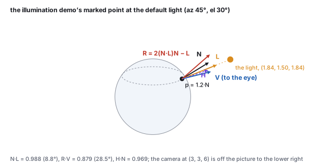
split of the vectors chapter, and works every number at the illumination demo’s marked point:
\(\mathbf{N}\cdot\mathbf{L} = 0.988\), \(\mathbf{R}\cdot\mathbf{V} = 0.879\), a specular factor of
\(0.879^{30} = 0.021\), Blinn’s \(\mathbf{H}\cdot\mathbf{N} = 0.969\), and the final color. It then covers
what the model needs around it: the correct transform for normals, the directional, point and spot
sources with their falloff, shadows as a visibility term, the error of treating a lamp as a point, the sum over several lights, what replaces the ambient constant (occlusion, spherical harmonics, image-based light), the tone-mapping step that fits an
unbounded brightness onto a display, and where in the pipeline the sum is paid for.
Definition (the shading vectors)
At a surface point \(\mathbf{p}\): \(\mathbf{N}\) is the unit surface normal (the vertex normal of
the meshes chapter, interpolated to the pixel); \(\mathbf{L}\) is the
unit vector from \(\mathbf{p}\) toward the light; \(\mathbf{V}\) is the unit vector from
\(\mathbf{p}\) toward the eye. A local illumination model computes the color at \(\mathbf{p}\) from
these three vectors and the material, and from nothing else in the scene.
The convention that \(\mathbf{L}\) points toward the light, not along the light’s travel, is what
makes “facing the light” mean \(\mathbf{N}\cdot\mathbf{L}\) near 1; a sign slip here inverts the
whole model. Because all three are unit vectors, every dot product below is the cosine of an angle
(the vectors chapter).
The word local is the model’s honest scope. It captures direct light: matte falloff,
highlights, per-light attenuation. It ignores everything that involves other surfaces: a red wall
tinting a white floor, soft shadows, a floor reflecting the room, the darkening in a crease. Those are
the global effects of the light-transport
chapter, and they cost tracing light around the scene. The local model buys a handful of dot
products per pixel with that omission, and one of its three terms exists only to apologize for it.
The worked instance throughout is the illumination demo’s: a sphere of radius 1.2 at the origin,
the camera at \((3, 3, 6)\), a point light on an orbit of radius 3 whose default position is azimuth
\(45^\circ\), elevation \(30^\circ\), and one marked point where the normal is
\(\mathbf{N} = \mathrm{normalize}(1, 1, 1) = (0.577, 0.577, 0.577)\). For a sphere at the origin the
outward normal at any point is the point normalized, so \(\mathbf{p} = 1.2\,\mathbf{N} = (0.693, 0.693, 0.693)\).
The five vectors at the marked point with the light at its default position. \(\mathbf{R}\) is the mirror image of \(\mathbf{L}\) about \(\mathbf{N}\); \(\mathbf{H}\) bisects \(\mathbf{L}\) and \(\mathbf{V}\). The camera is off the picture.
Worked example (the light and \(\mathbf{L}\))
Azimuth \(a\) and elevation \(e\) on an orbit of radius 3, the same spherical formula as the camera of
the viewing chapter:
\(\text{light} = 3\,(\cos e \sin a,\; \sin e,\; \cos e \cos a) = 3\,(0.6124, 0.5, 0.6124) = (1.837, 1.500, 1.837)\).
Then \(\text{light} - \mathbf{p} = (1.144, 0.807, 1.144)\), of length 1.808, so
\(\mathbf{L} = (0.633, 0.446, 0.633)\). The eye: \((3, 3, 6) - \mathbf{p} = (2.307, 2.307, 5.307)\), length 6.23,
\(\mathbf{V} = (0.370, 0.370, 0.852)\). \(\mathbf{V}\) does not change when the light moves.
2 · Diffuse: Lambert’s cosine
A matte surface (chalk, paper, plaster) scatters incoming light equally in every direction, so its
brightness does not depend on where the eye is. It depends only on how much light lands on each unit
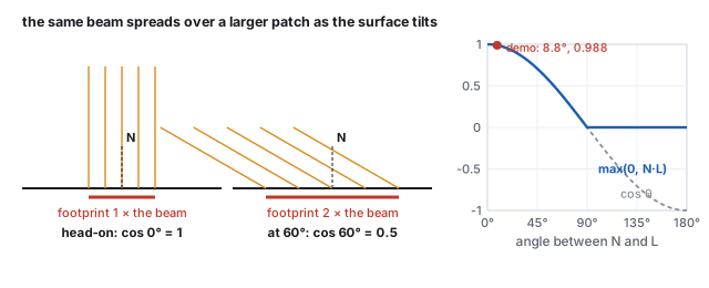
of area, and that is a projected-area question. A beam of fixed cross-section striking the surface
head-on covers a patch equal to its cross-section; striking at an angle \(\theta\) from the normal, the
same beam spreads over a patch \(1/\cos\theta\) times larger, so each unit of surface receives
\(\cos\theta\) of the head-on energy. Johann Heinrich Lambert measured this in 1760.
The same beam over a footprint \(1/\cos\theta\) times larger as the surface tilts, and the resulting factor \(\max(0, \mathbf{N}\cdot\mathbf{L})\), with the marked point at the default light marked.
Definition (the diffuse term)
\[
\text{diffuse} = k_d\, I_{\text{light}}\, \max(0,\; \mathbf{N}\cdot\mathbf{L}),
\]
with \(k_d\) the material’s diffuse reflectance (its base color, per channel; a texture supplies it
per pixel) and \(I_{\text{light}}\) the light’s color and intensity. The clamp is the back-face rule:
past \(90^\circ\) the cosine is negative, and a surface turned away from the light receives nothing, not
negative light.
Worked example (\(\mathbf{N}\cdot\mathbf{L}\) at the marked point)
With all three components of \(\mathbf{N}\) equal to 0.577,
\[
\mathbf{N}\cdot\mathbf{L} = 0.577\,(0.633 + 0.446 + 0.633) = 0.577 \times 1.712 = 0.988,
\]
an angle of \(8.8^\circ\): the marked point faces almost straight into the light, and the diffuse factor
is \(\max(0, 0.988) = 0.988\). Swing the light behind the sphere, to azimuth \(225^\circ\) and elevation
\(-30^\circ\): the light is at \((-1.837, -1.500, -1.837)\), \(\mathbf{L} = (-0.603, -0.523, -0.603)\), and
\(\mathbf{N}\cdot\mathbf{L} = -0.998\), nearly antiparallel. The clamp makes the diffuse factor exactly 0.
The demo’s panel prints both numbers.
This one clamped dot product is the workhorse of real-time shading; most of what makes a scene read as
lit is the diffuse term. Because the term is per channel, a red light on a white surface gives red
diffuse, and a white light on a red texture gives red diffuse too: \(k_d\) and \(I_{\text{light}}\)
multiply.
Irradiance, and why the diffuse constant is divided by \(\pi\)
Lambert’s factor is the geometry of one light. The same argument for all the light arriving at
the point is the irradiance, the cosine-weighted integral of the incoming radiance over the
hemisphere, \(E = \int_H L(\omega)\cos\theta\,d\omega\), in the units of
the color chapter. Under a sky of uniform radiance \(L\) it is
\(\pi L\), not \(2\pi L\): the cosine halves the hemisphere’s solid angle. A Lambertian surface
of albedo \(\rho\) sends that energy back out equally in all directions, and to send out no more
than it received its reflected radiance must be \(\rho E/\pi\). The physically normalized diffuse
term is therefore \((\rho/\pi)\,L\cos\theta\) per light, and the \(k_d\) of this chapter is that
\(\rho/\pi\) with the light’s intensity absorbed into the constant. Under the uniform sky a white
surface then reflects radiance \(\rho E/\pi = L\): exactly as bright as the sky, which is the check.
The light-transport chapter makes the same point for
every reflection model, and the \(\pi\) is the first thing to go wrong when a Phong shader is fed
physical light units.
3 · Specular: the mirror direction, Phong and Blinn
A glossy surface (plastic, wet paint, polished metal) adds a compact bright spot, the reflection of the
light source itself. Unlike diffuse it is view-dependent: the spot sits where the surface mirrors the
light toward this eye, and it slides as the eye moves. A perfect mirror shows the light only when the
eye is exactly on the mirror direction; a slightly rough surface spreads the spot around it.
The mirror direction
Reflecting \(\mathbf{L}\) about \(\mathbf{N}\) keeps its component along \(\mathbf{N}\) and negates the
component in the surface. With the projection split
\(\mathbf{L} = (\mathbf{N}\cdot\mathbf{L})\mathbf{N} + [\mathbf{L} - (\mathbf{N}\cdot\mathbf{L})\mathbf{N}]\),
\[
\mathbf{R} = (\mathbf{N}\cdot\mathbf{L})\mathbf{N} - [\mathbf{L} - (\mathbf{N}\cdot\mathbf{L})\mathbf{N}] = 2(\mathbf{N}\cdot\mathbf{L})\mathbf{N} - \mathbf{L}.
\]
It is unit when \(\mathbf{N}\) and \(\mathbf{L}\) are. Checks: \(\mathbf{L} = \mathbf{N}\) gives
\(\mathbf{R} = \mathbf{N}\) (a head-on ray reflects back); \(\mathbf{N}\cdot\mathbf{L} = 0\) gives
\(\mathbf{R} = -\mathbf{L}\) (a grazing ray continues, flipped).
Definition (the Phong specular term)
\[
\text{specular} = k_s\, I_{\text{light}}\, \max(0,\; \mathbf{R}\cdot\mathbf{V})^{s},
\]
with \(k_s\) the specular color (near white for plastics, since the highlight is the light’s color,
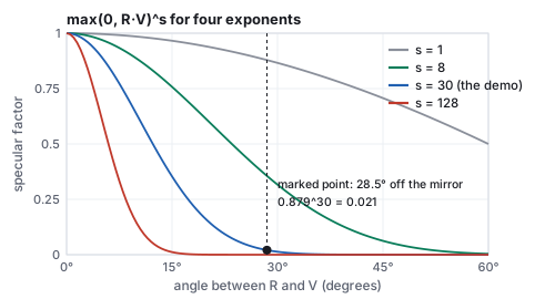
not the surface’s) and \(s\) the shininess exponent. Raising a cosine below 1 to a high power
collapses it: a large \(s\) is a tight highlight, a small \(s\) a broad sheen.
Worked example (\(\mathbf{R}\), \(\mathbf{R}\cdot\mathbf{V}\), and the exponent)
\(2(\mathbf{N}\cdot\mathbf{L}) = 1.977\), so \(2(\mathbf{N}\cdot\mathbf{L})\mathbf{N} = (1.141, 1.141, 1.141)\) and
\(\mathbf{R} = (1.141, 1.141, 1.141) - (0.633, 0.446, 0.633) = (0.508, 0.695, 0.508)\), which is unit.
Then
\[
\mathbf{R}\cdot\mathbf{V} = 0.508\cdot0.370 + 0.695\cdot0.370 + 0.508\cdot0.852 = 0.879,
\]
an angle of \(28.5^\circ\) between the mirror direction and the eye. The specular factor for several
exponents:
\(s\)
\(0.879^s\)
look
1
0.879
a broad wash, no visible spot
8
0.356
a soft sheen
30 (the demo)
0.021
a tight, plausible plastic highlight; the marked point is on its skirt
128
\(6.6\times10^{-8}\)
a pinpoint; nothing \(28^\circ\) off the mirror survives
\(0.021\) is the demo panel’s specular reading at the default shininess.
\(\max(0, \mathbf{R}\cdot\mathbf{V})^s\) against the angle to the mirror direction. The exponent sets the highlight’s width; the marked point sits \(28.5^\circ\) off the mirror direction.
Jim Blinn’s 1977 variant replaces the mirror test with a half-vector test. Let
\(\mathbf{H} = \mathrm{normalize}(\mathbf{L} + \mathbf{V})\), the direction bisecting light and eye; the
surface mirrors the light into the eye exactly when \(\mathbf{N} = \mathbf{H}\), so
\(\max(0, \mathbf{H}\cdot\mathbf{N})^s\) peaks in the same place as Phong’s term. It needs no
reflection vector, behaves better at grazing angles, and for a directional light and a distant eye
\(\mathbf{H}\) is constant over the whole surface; it is what most engines, three.js included, actually
compute. The two are not numerically equal.
Worked example (Blinn at the same point)
\(\mathbf{L} + \mathbf{V} = (1.003, 0.817, 1.485)\), length 1.97, \(\mathbf{H} = (0.509, 0.415, 0.754)\), and
\(\mathbf{H}\cdot\mathbf{N} = 0.577\,(0.509 + 0.415 + 0.754) = 0.969\). The half angle is roughly half the
mirror angle (\(14.3^\circ\) against \(28.5^\circ\)), so Blinn’s cosine is larger: at \(s = 30\),
\(0.969^{30} = 0.387\) against Phong’s 0.021. To match Phong’s value at this point Blinn needs
\(s = 123\), about four times the exponent, the usual rule of thumb. The demo’s panel computes
classic Phong while its material renders Blinn, so the printed \(\mathbf{R}\cdot\mathbf{V}\) and the rendered
highlight agree in position and in how they tighten with \(s\), not digit for digit.
Energy and the exponent
Raising the cosine to \(s\) narrows the highlight but also shrinks the total light it reflects: the
integral of \(\max(0, \mathbf{R}\cdot\mathbf{V})^s\) over the hemisphere is \(2\pi/(s + 2)\). A shader that
uses the raw term makes a smooth surface reflect less light than a rough one, for no physical
reason. The normalized Phong lobe multiplies by \((s + 2)/2\pi\): 5.09 at \(s = 30\), 20.7 at
\(s = 128\), so that a tighter highlight is a brighter one and the surface reflects the same total.
At the marked point the normalized specular factor is \(5.09 \times 0.021 = 0.107\) rather than
\(0.021\). Real materials behave this way (a polished apple has a small bright glint, a dull one a
wide dim sheen of the same total), and it is the first step from Phong toward the microfacet
models of the light-transport chapter, whose
normal-distribution term is a normalized lobe by construction.
4 · Ambient, and the whole sum
Both terms vanish where no light arrives directly, and a scene shaded by them alone has shadows of
pure black. Real shadows are not black; light bounces off every other surface and fills them, and that
is exactly what the local model refuses to compute. The ambient term stands in for all of it with
a constant, \(k_a\, I_{\text{ambient}}\), the same at every point regardless of direction. It has no
physical derivation; too much of it flattens the scene (every point gets the same floor and the shape
cues of the diffuse term wash out), too little makes shadows inky.
Definition (the Phong reflection model)
\[
\text{color} = k_a I_a \;+\; k_d I \max(0, \mathbf{N}\cdot\mathbf{L}) \;+\; k_s I \max(0, \mathbf{R}\cdot\mathbf{V})^s,
\]
per color channel, summed over the lights (Section 6), then fitted to the display (Section 8).
Bui Tuong Phong, 1975.
Worked example (the color at the marked point)
Take a red plastic: \(k_a = 0.12\), \(k_d = (0.86, 0.36, 0.30)\), \(k_s = 0.5\), \(s = 30\), a white light and
white ambient of intensity 1. Ambient: \(0.12\,k_d = (0.103, 0.043, 0.036)\). Diffuse:
\(0.988\,k_d = (0.850, 0.356, 0.297)\). Specular: \(0.5\times0.021 = 0.010\) on every channel. Sum:
\((0.964, 0.409, 0.343)\). The diffuse term dominates because the point faces the light; the specular
adds a hundredth because the point is on the skirt of the highlight, and it adds equally to all three
channels, which is why highlights on colored plastic are white.
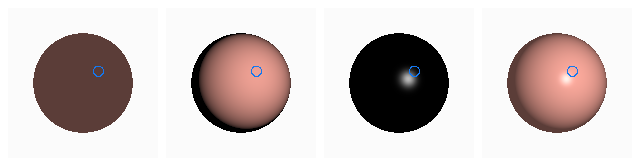
The demo’s sphere from the demo’s camera, ray-cast and shaded by this chapter’s formula one term at a time: ambient, diffuse, specular, and their sum. The blue ring marks the worked point; its pixel in the sum panel is \((0.964, 0.409, 0.343)\) before display encoding.
See it liveLight a sphere: one
sphere, one orbiting point light, and the marked point of this chapter, with the four scalars
\(\mathbf{N}\cdot\mathbf{L}\), \(\mathbf{R}\cdot\mathbf{V}\), diffuse and specular computed live in the course
library’s vector code. Drag the light behind the sphere and watch the diffuse clamp to zero; raise
the shininess and watch the highlight tighten.
Hands-on
Reproduce the demo’s panel from the library’s vector routines; the demo runs this same code:
Change light to \((-1.837, -1.5, -1.837)\) and confirm \(\mathbf{N}\cdot\mathbf{L} = -0.998\); then replace Math.pow(dot(R,V),30) by Math.pow(Math.max(0,dot(R,V)),30) and see why the clamp matters there.
Tabulate Reinhard in one line and compare with Section 8:
In the demo, orbit the camera (drag) with the light fixed until the panel’s \(\mathbf{R}\cdot\mathbf{V}\) reads its maximum: the eye is then on the mirror direction of the marked point, and the highlight sits on the marker. \(\mathbf{N}\cdot\mathbf{L}\) does not change while you do it.
Whether the sum is evaluated per vertex and interpolated (Gouraud) or per pixel from an interpolated
normal (Phong shading) is the choice shown in
the meshes chapter; the specular term is what makes the difference
visible.
5 · Normals under a transform
Every term above starts from \(\mathbf{N}\), and \(\mathbf{N}\) is stored in the model’s own frame.
Positions go to world space through the model matrix \(M\); normals must not. A normal is defined by
perpendicularity to the surface, and a non-uniform scale or a shear does not preserve right angles:
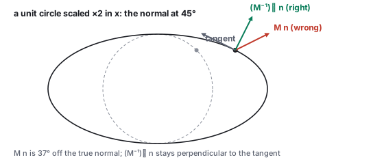
push the normal through \(M\) and it leans off the surface. The
affine chapter derives the rule; here is the figure and the number.
The normal matrix
If positions transform by \(M\) (its linear part \(A\)), normals transform by \((A^{-1})^{\top}\), then
renormalize. For a rotation \((A^{-1})^{\top} = A\) and nothing changes; the rule matters only under
scaling and shear, which is why the bug hides until someone squashes a model.
A unit circle scaled \(2\times\) in \(x\). At the point that was at \(45^\circ\), the normal pushed through \(M\) leans \(37^\circ\) off the true normal; the inverse transpose keeps it perpendicular to the tangent.
Worked example (the ellipse)
\(A = \mathrm{diag}(2, 1)\); the point \((0.707, 0.707)\) with normal \(\mathbf{n} = (0.707, 0.707)\) moves to
\((1.414, 0.707)\), where the ellipse’s tangent is \((-0.894, 0.447)\). Wrong: \(A\mathbf{n} = (1.414, 0.707)\),
normalized \((0.894, 0.447)\), whose dot with the tangent is \(-0.6\), not perpendicular. Right:
\((A^{-1})^{\top} = \mathrm{diag}(0.5, 1)\), \((0.354, 0.707)\), normalized \((0.447, 0.894)\), dot with the tangent
\(0\). The two candidates are \(36.9^\circ\) apart, and every cosine in the model is off by that much.
Engines compute the normal matrix once per object and pass it to the vertex shader. When a shader has
only \(M\), a serviceable substitute transforms two points, \(\mathbf{p}\) and \(\mathbf{p} + \mathbf{n}\),
and takes the normalized difference; for a rigid \(M\) it is exact, and under scaling it is an
approximation that improves as the step along the normal shrinks relative to the surface’s curvature.
6 · Light sources: directional, point, spot
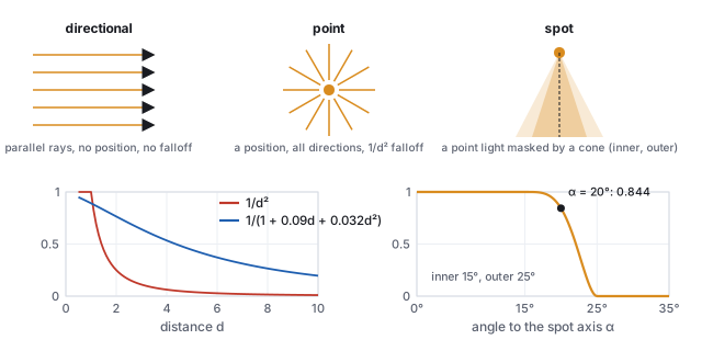
\(\mathbf{L}\) and \(I_{\text{light}}\) come from a light source, and engines have three kinds.
The three light types; distance attenuation, physical and tunable; and the spot cone with inner angle \(15^\circ\) and outer angle \(25^\circ\).
Directional (the sun): a direction and no position. \(\mathbf{L}\) is the same constant
vector at every point, and there is no falloff. Cheapest.
Point (a bulb): a position radiating in all directions. \(\mathbf{L}\) is computed per
point, as in Section 1, and the intensity falls with distance. A source of fixed power spreads over a
sphere of area \(4\pi d^2\), so the physical falloff is \(1/d^2\): twice the distance, a quarter of the
light. Engines often use a tunable \(1/(k_c + k_l d + k_q d^2)\) whose constant term keeps the value
finite at \(d = 0\), and a cutoff radius beyond which the light is skipped entirely.
\(d\)
\(1/d^2\)
\(1/(1 + 0.09d + 0.032d^2)\)
1
1
0.891
2
0.25
0.765
4
0.0625
0.534
10
0.01
0.196
Spot (a flashlight): a point light masked by a cone about an aim direction
\(\mathbf{D}\). With \(\alpha\) the angle between \(-\mathbf{L}\) and \(\mathbf{D}\), the mask is 1 inside an
inner angle \(\theta_{\min}\), 0 outside an outer angle \(\theta_{\max}\), and a smooth fade between,
multiplied into the light’s intensity. The classroom shader fades with
\(\mathrm{smoothstep}\bigl(1 - (\theta_{\min} - \alpha)^2 / (\theta_{\max} - \theta_{\min})^2\bigr)\), where
\(\mathrm{smoothstep}(t) = 3t^2 - 2t^3\). David Warn introduced the cone and its controls in 1983.
Worked example (the spot’s edge)
\(\theta_{\min} = 15^\circ\), \(\theta_{\max} = 25^\circ\), \(\alpha = 20^\circ\): \((15 - 20)^2 / 10^2 = 0.25\),
\(t = 0.75\), \(\mathrm{smoothstep}(0.75) = 3(0.5625) - 2(0.4219) = 0.844\). At \(18^\circ\) the mask is 0.977, at
\(22^\circ\) 0.515, at \(25^\circ\) 0: a soft penumbra ten degrees wide.
The model is linear in the light, so several lights simply add: each contributes its own diffuse and
specular with its own \(\mathbf{L}\), \(\mathbf{R}\), color and attenuation, and the ambient term is added
once. A second light at azimuth \(200^\circ\), elevation \(20^\circ\), at half intensity, sees the marked
point with \(\mathbf{N}\cdot\mathbf{L}_2 = -0.719\): its contribution there is zero, and the total diffuse
stays 0.988. The cost is lights times shaded pixels, which is why real-time engines cap how many lights
touch each object or restructure the loop (deferred and clustered shading) to keep it bounded.
Shadows: the visibility term
Nothing in the sum so far asks whether the light can see the point. A local model adds a
visibility factor \(V_i \in [0, 1]\) per light, multiplying that light’s diffuse and
specular terms, and computes it one of two ways: a shadow ray toward the light, as
the ray-tracing chapter does, or a shadow map, the
light’s depth buffer compared per pixel, worked in
the texture chapter. A point light gives a hard
edge; an area light gives a penumbra, which a shadow map approximates by filtering several depth
comparisons and a ray tracer by sampling the light’s area. The ambient term is deliberately
not multiplied by \(V\): it stands for the light that arrives around the occluder.
Area lights and the point-light approximation
No real source is a point. A ceiling panel, a window, the sun’s disk all subtend an angle, and
the point-light formula is their limit as the distance grows. The error is largest where lights are
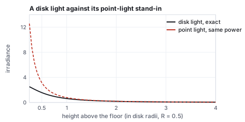
usually placed, close to the surface. For a disk of radius \(R\) and radiance \(L\) facing a point on
its axis at height \(h\), the exact irradiance is \(E = \pi L R^2/(h^2 + R^2)\); a point light of the
same total power gives \(\pi L R^2/h^2\).
A disk light and its point-light stand-in. Beyond two radii the two agree within 6 %; at half a radius the point light is twice too bright, and at a quarter, five times.
Worked example (how close is too close)
\(R = 0.5\), \(L = 1\):
\(h\)
0.25
0.5
1
2
4
disk, exact
2.513
1.571
0.628
0.185
0.048
point light
12.566
3.142
0.785
0.196
0.049
ratio
5.0
2.0
1.25
1.06
1.02
A lamp shade of radius 0.5 half a unit above a table is twice as bright under the point model as in
life, and its highlight is a dot rather than a reflection of the shade. Real-time engines now
evaluate sphere, disk and rectangle lights analytically (linearly transformed cosines, Heitz and
others 2016) for the diffuse and specular terms; the point light survives as the cheap case and
for sources small enough that the ratio is 1.
Pitfall
The inverse-square law applies to a point. Applying it to an area light close to a surface
produces the blown-out hot spot of the table’s first column, and the usual response, adding a
constant to the denominator (Section 6’s polynomial), fixes the symptom by making the falloff
wrong everywhere. The honest fix is the area formula, whose denominator \(h^2 + R^2\) is the
inverse-square law with the light’s own size as the floor. At \(h = R\) it says the irradiance is
half of what a point light claims; no polynomial with fixed coefficients reproduces that for every
\(R\).
7 · Better than ambient: occlusion, harmonics, image-based light
The ambient constant fails in two directions: it lights creases and undersides as brightly as
exposed faces, and it has one color for every direction. Three techniques repair it while staying
local in cost, and together they are how real-time renderers approximate the indirect light of
the rendering equation.
Definition (ambient occlusion)
The fraction of the cosine-weighted hemisphere above a point that is not blocked by nearby
geometry, \(A = \frac{1}{\pi}\int_H V(\omega)\cos\theta\,d\omega\), multiplied into the ambient term.
It is a purely geometric quantity, independent of the lights, and can be baked per vertex or
texel, or estimated per frame from the depth buffer (screen-space ambient occlusion).
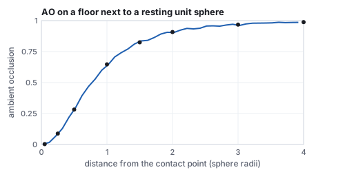
Occlusion on a floor beside a resting unit sphere, from 4,000 cosine-weighted rays per point. The contact shadow that a constant ambient cannot produce.
Worked example (a crease and a contact)
A point on the floor of a \(90^\circ\) crease sees exactly half its hemisphere: \(A = 0.5\) at the
corner, rising to 1 away from it. Beside a unit sphere resting on the floor, sampling the hemisphere
with 4,000 cosine-weighted rays gives \(A = 0.003\) at 0.05 radii from the contact, 0.28 at half a
radius, 0.65 at one, 0.91 at two, 0.99 at four. Multiplied into the ambient term of Section 4, the
sphere sits on a dark ring instead of floating on a uniformly lit floor.
Definition (spherical-harmonic irradiance)
Directional ambient light: the sky’s radiance \(L(\omega)\) is projected onto the spherical
harmonics, \(L_{lm} = \int L(\omega)\,Y_{lm}(\omega)\,d\omega\), and the irradiance for a normal
\(\mathbf{n}\) is \(E(\mathbf{n}) = \sum_{lm} A_l\,L_{lm}\,Y_{lm}(\mathbf{n})\) with
\(A_0 = \pi\), \(A_1 = 2\pi/3\), \(A_2 = \pi/4\) (Ramamoorthi and Hanrahan, 2001). The cosine lobe is
so smooth that 9 coefficients (\(l \le 2\)) capture the irradiance of any sky within about 1 %.
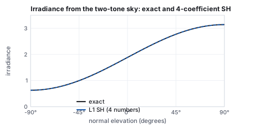
The two-tone sky of the light-transport chapter’s sphere grid, its irradiance computed exactly and from four spherical-harmonic numbers. For a sky that is constant on each side of the horizon the four are exact.
Worked example (four numbers for a sky, nine for a sun)
A sky of radiance 1 above the horizon and 0.2 below projects to \(L_{00} = 2.127\),
\(L_{1,-1} = 1.228\) (the \(y\) term) and zero for the two horizontal terms. Irradiance for the
marked normal (elevation \(35.3^\circ\)) is \(\pi(2.127)(0.2821) + \tfrac{2\pi}{3}(1.228)(0.4886)(0.577) = 2.61\),
the same as the hemisphere integral, because this sky’s irradiance is exactly
\(\pi L(1 + \cos\theta)/2\) per half, linear in the cosine, which the four coefficients span. Add a
sun, radiance 30 within \(10^\circ\) of the demo’s default light direction, and the four are not
enough:
normal
exact
4 coefficients
9 coefficients
toward the sun
5.340
4.639
5.509
the marked normal
5.425
4.730
5.589
straight up
4.554
4.560
4.451
away from the sun
1.257
0.555
1.425
Nine coefficients bring the worst case from 56 % low to 13 % high; a sun that sharp is better
handled as a directional light with the harmonics carrying the sky, which is the usual split.
Image-based lighting takes the same idea to a captured environment: a high-dynamic-range
panorama (a light probe, Debevec 1998) is stored as the cube map of
the texture chapter; its diffuse contribution is the
nine harmonics above, or a cube map pre-convolved with the cosine, read by the normal; its glossy
contribution is the same map pre-convolved with the specular lobe at several widths, stored in the
mip levels, read by the reflection vector at the level the roughness selects. Every pixel then sees
the whole environment in two texture fetches, which is why a rendered car in a photographed street
matches the street. The assumptions are the cube map’s: the environment is distant and nothing in
the scene occludes it, which ambient occlusion patches.
8 · Brightness has no ceiling: tone mapping
Several lights and a bright specular push the computed sum past 1, and that is correct: real
luminance spans many orders of magnitude, and a lighting sum is naturally high dynamic range.
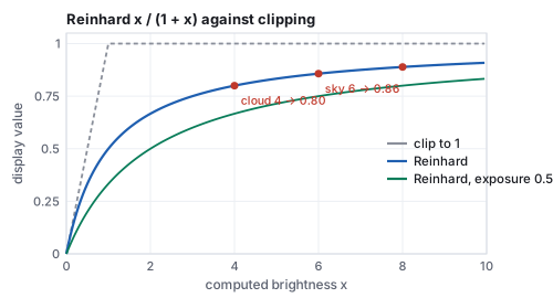
The display is not; it shows \([0, 1]\), where 1 is its brightest white. Clipping everything above 1
turns a sky at 6, a cloud at 4 and the sun at 40 into the same white, every distinction gone. A
tone-mapping curve compresses the unbounded range into \([0, 1)\) while keeping bright values
ordered.
Reinhard’s \(x/(1+x)\) against clipping, and the same curve at half exposure. Values that clipping would merge stay distinct.
Worked example (Reinhard)
The simplest respectable curve (Reinhard, Stark, Shirley and Ferwerda, 2002) is \(x/(1 + x)\):
\(x\)
0.25
0.5
1
2
4
8
40
\(x/(1+x)\)
0.200
0.333
0.500
0.667
0.800
0.889
0.976
Small values pass nearly unchanged, so shadows and midtones keep their look; large values are squeezed
toward 1 without reaching it. Cloud, sky and sun become 0.800, 0.857 and 0.976, three distinct grays where
clipping gave three whites. An exposure factor scales \(x\) first and chooses what counts as
middle gray: at exposure 0.5 the sun maps to \(20/21 = 0.952\) and the sky to \(3/4 = 0.75\). Production
pipelines use steeper film-like curves (the ACES curve is the common one), and all of them go last,
after every light has been summed, right before the value is written to the framebuffer and encoded for the display with the sRGB curve of
the color chapter. Every term of this chapter is computed in linear
light, on textures decoded from sRGB; the encoding happens once, after the tone map, and a shader that
lights undecoded textures or blends encoded values gets the dark, muddy result that chapter works
out.
9 · Shading cost: per vertex, per pixel, deferred
The sum is evaluated somewhere, and where decides the bill. Per vertex (Gouraud), it runs once per
vertex and the rasterizer interpolates colors: the full bunny is 35,947 evaluations regardless of
how large it is on screen. Per pixel (Phong shading), it runs once per covered pixel per triangle:
a bunny covering 250,000 pixels is 250,000 evaluations, seven times more, and with an overdraw of
3 (each pixel covered by three fragments before the depth test settles) 750,000.
Worked example (32 lights at 1080p)
Forward shading with 32 lights, overdraw 3, and 120 operations per light evaluation:
\(2{,}073{,}600 \times 3 \times 32 = 2.0\times10^8\) evaluations, \(2.4\times10^{10}\) operations per
frame. Deferred shading first rasterizes the scene into a geometry buffer (position or depth,
normal, albedo, roughness: about 20 bytes per pixel, 41.5 MB at 1080p) with no lighting, then
shades each pixel once from the buffer: \(2{,}073{,}600 \times 32 = 6.6\times10^7\) evaluations,
the overdraw factor gone. Tiled deferred shading goes further: divide the screen into
\(16\times16\) tiles (8,160 of them), find the lights that reach each tile, typically 6 rather
than 32, and shade each pixel against only those: \(1.2\times10^7\) evaluations, sixteen times
fewer than forward. The price is the buffer’s bandwidth, one material model for the whole
screen, and the loss of hardware multisampling at edges, which is why forward+ (the tile culling
with forward shading) is the other common design.
scheme
lighting evaluations per frame
memory
limits
Gouraud
vertices
none
highlights between vertices lost
forward, per pixel
pixels × overdraw × lights
none
every fragment pays for every light
deferred
pixels × lights
G-buffer, 41.5 MB at 1080p
one material model, no MSAA, no transparency
tiled deferred
pixels × lights per tile
G-buffer + light lists
as deferred
10 · Where the local model ends
The Phong model is a description of what shading looks like, not of what light does. Its specular
lobe is not energy-conserving (a high exponent reflects less total light than a low one, for no
physical reason), its ambient term is a confession, and it has no notion of a surface being metal or
dielectric beyond the color of \(k_s\). The light-transport
chapter replaces the sum with the rendering equation and the specular term with a microfacet
model whose parameters (roughness, metalness) mean something measurable, and
the learned-scenes chapter dispenses with the surface altogether. The
three vectors, the cosine, and the clamp survive every one of those upgrades.
Papers
J. H. Lambert, Photometria, 1760. H. Gouraud, “Continuous Shading of Curved Surfaces,”
IEEE Transactions on Computers C-20(6), 1971. B. T. Phong, “Illumination for Computer Generated
Pictures,” Communications of the ACM 18(6), 1975. J. Blinn, “Models of Light Reflection for
Computer Synthesized Pictures,” SIGGRAPH 1977. D. Warn, “Lighting Controls for Synthetic
Images,” SIGGRAPH 1983. E. Reinhard, M. Stark, P. Shirley and J. Ferwerda, “Photographic Tone
Reproduction for Digital Images,” SIGGRAPH 2002. R. Ramamoorthi and P. Hanrahan, “An Efficient
Representation for Irradiance Environment Maps,” SIGGRAPH 2001. P. Debevec, “Rendering Synthetic
Objects into Real Scenes,” SIGGRAPH 1998 (light probes). E. Heitz, J. Dupuy, S. Hill and D. Neubelt,
“Real-Time Polygonal-Light Shading with Linearly Transformed Cosines,” SIGGRAPH 2016. M. Deering,
S. Winner, B. Schediwy, C. Duffy and N. Hunt, “The Triangle Processor and Normal Vector Shader,”
SIGGRAPH 1988 (deferred shading).
11 · Exercises
Exercise 1 (diffuse)
Move the demo’s light to azimuth \(90^\circ\), elevation \(0^\circ\) (on the \(x\) axis). Compute \(\mathbf{L}\) and the diffuse factor at the marked point.
Solution
Light at \((3, 0, 0)\); \(\text{light} - \mathbf{p} = (2.307, -0.693, -0.693)\), length 2.507, \(\mathbf{L} = (0.920, -0.276, -0.276)\); \(\mathbf{N}\cdot\mathbf{L} = 0.577\,(0.920 - 0.276 - 0.276) = 0.212\), an angle of \(77.8^\circ\). The point is lit, dimly: a fifth of full brightness.
Exercise 2 (the mirror direction)
For \(\mathbf{N} = (0, 1, 0)\) and \(\mathbf{L} = (0.6, 0.8, 0)\), compute \(\mathbf{R}\) and verify it is unit and makes the same angle with \(\mathbf{N}\) as \(\mathbf{L}\) does.
Solution
\(\mathbf{N}\cdot\mathbf{L} = 0.8\); \(\mathbf{R} = 1.6\,(0, 1, 0) - (0.6, 0.8, 0) = (-0.6, 0.8, 0)\); length \(\sqrt{0.36 + 0.64} = 1\); \(\mathbf{R}\cdot\mathbf{N} = 0.8 = \mathbf{L}\cdot\mathbf{N}\). The in-surface component flipped sign, the along-normal component did not.
Exercise 3 (shininess)
An eye \(10^\circ\) off the mirror direction. What specular factor at \(s = 30\), and what exponent would halve it?
Solution
\(\cos 10^\circ = 0.985\); \(0.985^{30} = 0.633\). Halving needs \(0.985^s = 0.316\), \(s = \ln 0.316 / \ln 0.985 = 75\). Doubling the exponent roughly squares the factor, so the highlight’s width shrinks like \(1/\sqrt{s}\).
Exercise 4 (Blinn)
Show that \(\mathbf{H}\cdot\mathbf{N} = 1\) exactly when \(\mathbf{R} = \mathbf{V}\).
Solution
\(\mathbf{H} = \mathbf{N}\) means \(\mathbf{L} + \mathbf{V}\) is along \(\mathbf{N}\), so \(\mathbf{V}\) and \(\mathbf{L}\) have opposite in-surface components and equal along-normal components (both unit): \(\mathbf{V} = 2(\mathbf{N}\cdot\mathbf{L})\mathbf{N} - \mathbf{L} = \mathbf{R}\). Conversely \(\mathbf{R} = \mathbf{V}\) gives \(\mathbf{L} + \mathbf{V} = 2(\mathbf{N}\cdot\mathbf{L})\mathbf{N}\), along \(\mathbf{N}\). The two highlights peak at the same place.
Exercise 5 (attenuation)
A point light of intensity 1 at distance 4 under \(1/d^2\) falloff, and the same light under the polynomial of Section 6. How much brighter must the physical light be to match the polynomial’s value at \(d = 4\)?
Solution
\(1/16 = 0.0625\) against \(0.534\): a factor of \(8.5\). The polynomial is not physics; it is an artist’s falloff that keeps distant objects readable without a light bright enough to blow out near ones.
Exercise 6 (tone mapping)
Two pixels compute to 3 and 30. What is their ratio on screen after clipping, after Reinhard, and after Reinhard at exposure 0.1?
Solution
Clipping: both 1, ratio 1. Reinhard: \(0.75\) and \(0.968\), ratio 1.29. Exposure 0.1: \(0.3 \mapsto 0.231\) and \(3 \mapsto 0.75\), ratio 3.25. Lower exposure spends more of the display range on the bright end; the ratio of 10 is never recovered, since that is what compression means.
Exercise 7 (normalization)
A white Lambertian wall (\(\rho = 1\)) under a uniform overcast sky of radiance \(L = 2\). What is its irradiance and its outgoing radiance? What does a shader with \(k_d = 1\) and no \(\pi\) report if it treats the sky as a single light of intensity 2 from straight above?
Solution
\(E = 2\pi = 6.28\); outgoing radiance \(\rho E/\pi = 2\), the sky’s own. The unnormalized shader gives \(k_d \cdot 2 \cdot \cos 0 = 2\), which happens to agree because the whole sky was collapsed to one direction; tilt the wall \(60^\circ\) and the shader gives 1 while the true value stays 2 (a uniform sky lights every orientation equally): the collapse, not the \(\pi\), is the error there.
Exercise 8 (an area light)
A square ceiling panel of side 0.6 m and radiance 5 lights a desk 1.5 m below its center. Estimate the irradiance with the disk formula of equal area, and with a point light of equal power. Is the point light acceptable?
Solution
Equal-area disk: \(R = 0.6/\sqrt\pi = 0.339\); \(E = \pi\cdot5\cdot0.115/(2.25 + 0.115) = 0.763\). Point: \(\pi\cdot5\cdot0.115/2.25 = 0.802\), 5 % high. Acceptable at that distance; at 0.3 m below the panel the ratio would be \((0.09 + 0.115)/0.09 = 2.3\).
Exercise 9 (harmonics)
Using the four coefficients of Section 7, compute the irradiance for a normal pointing straight down and check it against \(\pi \cdot 0.2\).
Solution
\(Y_{00} = 0.2821\), \(Y_{1,-1}(\mathbf{n}) = 0.4886\,n_y = -0.4886\): \(E = \pi(2.127)(0.2821) + \tfrac{2\pi}{3}(1.228)(-0.4886) = 1.885 - 1.257 = 0.628 = 0.2\pi\). A downward normal sees only the ground’s radiance 0.2 over its whole hemisphere.
Exercise 10 (shading cost, demo)
Open the illumination demo, set shininess to 128, and orbit until the highlight is a pinpoint. Estimate how many pixels it covers, and from that how many of the sphere’s vertices (a default sphere of 32 by 16 segments has about 500) would have to fall inside it for Gouraud shading to show it at all.
Solution
At \(s = 128\) the highlight is a few dozen pixels across on a sphere of a few hundred pixels: it covers under 1 % of the sphere’s area, and with about 500 vertices spread over the visible half (250), the expected number inside it is 1 or 2. Gouraud shading would show the highlight only when a vertex happens to sit in it, and it would flicker as the sphere turns, the failure the meshes chapter’s middle sphere shows.