This chapter links to the course’s interactive demos and uses MathJax for its formulas. Read it through the course website (or download the file and open it in a browser); a Canvas inline preview will reach neither the demos nor the math. All chapters.
Polygonal Meshes: Building, Shading, and Simplifying Surfaces
The Digital Michelangelo Project's raw scan of the David holds 2 billion polygons. Levoy et al., The Digital Michelangelo Project, SIGGRAPH 2000
Every real-time surface is a triangle mesh: a list of vertex positions and a list of index triples, nothing more. This chapter builds one from scratch, the \(2\times2\) grid the mesh-grid demo constructs, and works every number on it: the row-major index formula, the counts \((n+1)^2\), \(2n^2\) and \(6n^2\), the face normal of one triangle as a cross product, the averaged normal at a shared vertex, and what happens to all of them when the center vertex is lifted. It then turns to what the index array says about the surface as a whole: the half-edge structure that makes adjacency queries constant-time, Euler’s formula and manifoldness checked on the bunny, and the valence histogram. It shows the same surface shaded three ways, sweeps a profile curve into a surface of revolution, extracts a mesh from a scalar field with marching cubes, and closes with the reverse problem: taking triangles away. An edge collapse is worked with the quadric error metric on the lifted grid, and the Stanford bunny’s measured level-of-detail ladder gives the distance rule that decides which version to draw.
- A surface is two arrays
- Building a grid from a formula
- Adjacency: the half-edge structure
- Topology: Euler’s formula, manifolds, valence
- Face normals and vertex normals
- Flat, Gouraud, and Phong shading
- Editing: move a vertex, recompute
- Sweeping a profile
- Surfaces from volumes: marching cubes
- Simplification: the edge collapse and the quadric error
- Levels of detail and progressive meshes
- Mesh files: OBJ and glTF
- Exercises
1 · A surface is two arrays
Two facts of geometry make the triangle the hardware primitive. Three points always lie in one plane, so a triangle is flat and has one unambiguous normal; a quadrilateral’s four corners need not be coplanar, and a bent quad has no single normal and no single interior. A triangle is also always convex, so filling it is the fixed edge-function loop of the rasterization chapter, the same loop for every triangle ever drawn. Anything else is cut into triangles first.
The indirection is what makes the representation efficient. In a grid every interior vertex belongs to six triangles. Stored once and referenced six times, its position, its normal and its texture coordinate live in one place; move it and all six triangles follow. Without indices the same vertex would be copied six times and a modeling tool would have to find and edit every copy. The GPU receives the two arrays as they are: a vertex buffer and an index buffer.
Winding is not cosmetic. The renderer usually skips back faces (a closed solid never shows its inside), so a triangle listed in the wrong order disappears; and, as Section 5 shows, the sign of the computed normal is the winding, so a wrong order also lights the surface from inside.
2 · Building a grid from a formula
The mesh-grid demo builds an \(n\times n\) grid of quads on the \(xz\) plane, spanning \([-1.5, 1.5]\) on both axes, and splits each quad into two triangles. With \(n\) quads per side there are \(n+1\) lattice points per side, numbered row by row (row along \(z\), column along \(x\)): \[ \mathrm{index}(\mathrm{row}, \mathrm{col}) = \mathrm{row}\cdot(n+1) + \mathrm{col}, \qquad \mathbf{v}_{\mathrm{index}} = \bigl(-1.5 + \mathrm{col}\cdot\tfrac{3}{n},\; 0,\; -1.5 + \mathrm{row}\cdot\tfrac{3}{n}\bigr). \] The quad at \((\mathrm{row}, \mathrm{col})\), for \(0 \le \mathrm{row}, \mathrm{col} < n\), has corners \(v_{00} = \mathrm{index}(\mathrm{row}, \mathrm{col})\), \(v_{10} = \mathrm{index}(\mathrm{row}+1, \mathrm{col})\), \(v_{01} = \mathrm{index}(\mathrm{row}, \mathrm{col}+1)\), \(v_{11} = \mathrm{index}(\mathrm{row}+1, \mathrm{col}+1)\), and is cut along the \(v_{10}\)–\(v_{01}\) diagonal: \[ \text{tri}_0 = (v_{00}, v_{10}, v_{01}), \qquad \text{tri}_1 = (v_{01}, v_{10}, v_{11}), \] both counter-clockwise seen from \(+y\), so both front faces point up.
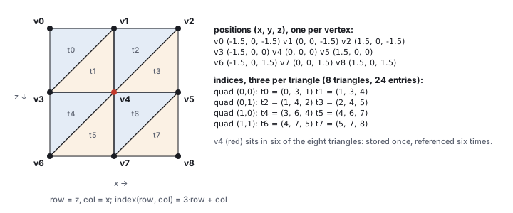
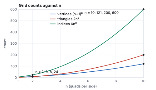
The construction reads off the three counts for any \(n\): \((n+1)^2\) vertices (fence posts, one more than the gaps), \(2n^2\) triangles (two per quad), \(6n^2\) index entries. At \(n = 2\): 9, 8, 24. At \(n = 10\): 121, 200, 600. At \(n = 100\): 10,201 vertices and 20,000 triangles. Vertices grow like triangles, half as fast in the limit: every vertex of a large grid is shared by six triangles, and every triangle has three corners, so \(T \approx 2V\), which holds for any large closed triangle mesh, not only grids.
3 · Adjacency: the half-edge structure
Two flat arrays answer one question quickly, which triangle has which corners, and no other. Every operation of Sections 5 to 11 asks the others: which triangles touch this vertex, which triangle is across this edge, which vertices ring this one. Searching the index array for each answer costs \(O(T)\) per query. A mesh that is edited, smoothed or simplified needs the answers in \(O(1)\), and the standard way to store them is the half-edge structure.
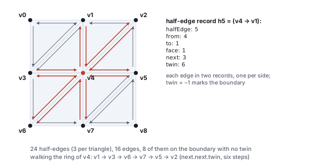
Building the structure from the two arrays is one pass over the triangles, hashing each directed edge \((a, b)\) to find its twin \((b, a)\): \(O(T)\) time and about 4 integers per half-edge, so roughly 12 integers per triangle on top of the 3 in the index array. The structure fails on exactly the meshes Section 4 calls non-manifold: an edge with three faces has no single twin. Alternatives store less (a vertex-to-triangle list, enough for normals and one-rings) or more (the winged-edge and quad-edge structures); the half-edge is the one in the libraries (OpenMesh, CGAL, Blender’s BMesh) because every query of this chapter is a constant number of pointer follows.
css551/); each prints what the text quotes.
- The face normal of \(\text{tri}_0\) and the unit normal of the lifted \(\text{tri}_1\), from the library’s own cross product:
node -e "import('./lib/core/xform.js').then(x=>{console.log(JSON.stringify(x.cross([0,0,1.5],[1.5,0,0])), JSON.stringify(x.normalize(x.cross([-1.5,0,1.5],[0,0.4,1.5]))))})" [0,2.25,0] [-0.2495,0.9357,-0.2495] (printed to 16 digits) - Count the bunny’s edges by hashing every directed edge, the first pass of a half-edge build, on the 868-triangle level:
node --input-type=module -e " import { readFileSync } from 'node:fs'; import { parseMeshBin } from './lib/core/models.js'; const b = readFileSync('lib/assets/models/bunny.l0.mesh.bin'); const m = parseMeshBin(b.buffer.slice(b.byteOffset, b.byteOffset + b.byteLength)); const cnt = new Map(); for (let t = 0; t < m.indices.length; t += 3) for (let k = 0; k < 3; k++) { const a = m.indices[t + k], c = m.indices[t + (k + 1) % 3]; const key = a < c ? a + '-' + c : c + '-' + a; cnt.set(key, (cnt.get(key) || 0) + 1); } console.log('V', m.positions.length / 3, 'E', cnt.size, 'F', m.indices.length / 3, 'chi', m.positions.length / 3 - cnt.size + m.indices.length / 3, 'boundary', [...cnt.values()].filter((c) => c === 1).length);" V 454 E 1325 F 868 chi -3 boundary 46Changel0tol3for the full mesh (35,947 declared vertices, of which 1,113 are referenced by no triangle; Section 4 explains the count). - In the mesh-grid demo, set \(n = 2\), turn on the normals overlay and drag the lift to 0.4: the six arrows around the center tilt inward and the center arrow stays vertical, the numbers of Section 5.
4 · Topology: Euler’s formula, manifolds, valence
The index array also fixes what kind of surface the mesh is, independently of where the vertices sit. Three facts about it can be checked in one pass and catch most broken meshes.
| mesh | \(V\) | \(E\) | \(F\) | \(\chi\) | boundary edges, loops | reading |
|---|---|---|---|---|---|---|
| cube | 8 | 12 | 6 | 2 | 0, 0 | closed, genus 0 |
| the \(2\times2\) grid | 9 | 16 | 8 | 1 | 8, 1 | a disk: \(2 - 0 - 1\) |
| icosphere, 320 faces | 162 | 480 | 320 | 2 | 0, 0 | closed, genus 0; \(E = 3F/2\) |
| bunny, full | 34,834 | 104,288 | 69,451 | \(-3\) | 223, 5 | \(2 - 2g - 5 = -3\): genus 0 with five holes |
| bunny, L0 | 454 | 1,325 | 868 | \(-3\) | 46, 5 | the same topology after simplification |
Two consequences matter in practice. Consistent orientation is checked by the twin rule: an interior edge whose two half-edges run the same direction means one of the two faces has its winding reversed, and its normal points the wrong way. And on a closed manifold every vertex’s faces sum, by the divergence theorem, to zero total vector area; a nonzero sum is a hole.
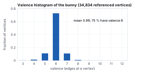
Valence, the number of edges at a vertex, is the local face of Euler’s formula: on a closed triangle mesh it averages \(6 - 12/V\), so nearly 6, and the bunny’s mean is 5.99 with 75 % of vertices at exactly 6. Vertices far from 6 are where subdivision (see the curves chapter) loses smoothness and where simplifiers produce slivers; a remesher’s job is largely to push the histogram toward that one bar. The triangle-quality measures of Section 11 (aspect ratio, the smallest angle) are the other half of mesh quality; valence is the combinatorial half.
5 · Face normals and vertex normals
Positions fix a surface’s shape and say nothing about which way it faces. Lighting (see the illumination chapter) needs the facing direction at every point, the unit normal, so every vertex carries one next to its position. For a mesh built by hand, the normals are computed from the positions, and the tool is the cross product of the vectors chapter.
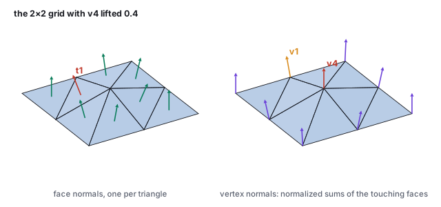
Two implementation notes. The accumulation runs once over the triangles, adding each face normal into its three vertices, then once over the vertices to normalize, so it costs \(O(T + V)\). And the normalize step needs a guard: a vertex whose incident faces have zero total area (a degenerate triangle, or the pole of Section 8) has a zero sum, and normalizing it produces NaN, which propagates through the lighting as black or garbage pixels. The demo returns \((0, 1, 0)\) when the sum’s length is below \(10^{-8}\).
Hard edges and split normals
Averaging assumes the surface is smooth across every edge. A cube averaged this way gets one normal per corner, the diagonal \((1, 1, 1)/\sqrt3\), and shades as a rounded blob with its edges washed out. The fix is to decide, per edge, whether it is smooth or hard: an edge whose two face normals differ by more than a threshold angle (Maya’s and Blender’s default is \(30^\circ\)) keeps separate normals on each side. Since a vertex holds one normal, a hard edge requires the vertex to be split: duplicated in the array, once per smooth group, with the same position and different normals. A cube shaded correctly has 24 vertices, not 8; the flat sphere of Section 6 is the extreme case with \(3T\) vertices and every edge hard. The same split is forced by texture seams, where one position needs two coordinates. The half-edge structure of Section 3 is built on the unsplit mesh, and the split copy is what goes to the GPU.
6 · Flat, Gouraud, and Phong shading
The averaging of Section 5 is also a choice of look. The same 80-triangle sphere is shown below three times, with identical positions and identical light; only what is interpolated across each triangle differs. The lighting formula is the Phong model of the illumination chapter; here it is a black box that turns a normal into a color.
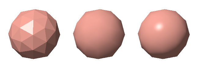
- Flat shading gives every pixel of a triangle the color computed from the face normal. It needs the face normal per triangle, which means vertices cannot be shared (a shared vertex can hold only one normal), so a flat-shaded mesh stores \(3T\) vertices. It is the deliberate low-poly look.
- Gouraud shading (Henri Gouraud, 1971) evaluates the lighting at each vertex with the averaged vertex normal and lets the rasterizer interpolate the resulting colors with the barycentric weights of the rasterization chapter. Three lighting evaluations per triangle instead of one per pixel. Its failure is visible in the middle panel: a highlight narrower than a triangle is lost if it falls between vertices, and it flickers as the object rotates and the highlight crosses vertices.
- Phong shading (Bui Tuong Phong, 1975) interpolates the normals instead, renormalizes the interpolated vector at each pixel (a blend of unit vectors is shorter than one), and evaluates the lighting per pixel. It is what every fragment shader does today; the cost that made it expensive in 1975 is now one dot product per pixel among many.
The word Phong names two different things: the interpolation scheme here and the reflection model in the illumination chapter. Both are from the same 1975 paper.
7 · Editing: move a vertex, recompute
A polygon modeling tool is the demo’s lift slider generalized: grab any vertex, move it, and rebuild what depends on it. Positions and normals are coupled. Moving one vertex changes the plane of every triangle that touches it, and therefore the face normals of those triangles and the averaged normals of every vertex on them, the one-ring neighborhood. A tool that moves a vertex and leaves the normals alone lights the surface as if it were still flat; the tent in the demo would render as a uniformly lit plane with a bump you could see only on the silhouette.
The update loop of a small editor reads every handle position into the vertex array, recomputes all normals, and hands both arrays back to the geometry each frame. For a mesh of a few hundred vertices that is cheap; a production editor recomputes only the one-ring of the moved vertex, which is why mesh data structures with adjacency (which triangles touch this vertex, which triangles share this edge) exist. The two flat arrays of Section 1 answer neither question without a search.
Deformations that move many vertices at once follow the same rule with a formula in place of a hand: a displacement field, a lattice, a skeleton (see the animation chapter). Every one of them ends in the same recompute-the-normals step.
Smoothing: the Laplacian
8 · Sweeping a profile
Placing vertices one by one does not scale. A surface of revolution generates a whole mesh from a short curve: a profile of \(P\) points \(\mathbf{p}_i = (r_i, y_i)\) in a half-plane, spun about the \(y\) axis in \(S\) equal steps. The vertex at (profile point \(i\), step \(j\)) is \[ \mathbf{v}(i, j) = R_y\!\left(\tfrac{2\pi j}{S}\right) (r_i, y_i, 0)^{\!\top} = \bigl(r_i \sin\theta_j,\; y_i,\; r_i \cos\theta_j\bigr), \qquad \theta_j = \tfrac{2\pi j}{S}, \] with \(R_y\) the rotation matrix of the rotation chapter. The \(P\times S\) vertices form a grid exactly like Section 2’s, indexed \(i\cdot S + j\), with one change: the column index wraps, \(j + 1\) taken modulo \(S\), so the last step connects back to the first and the surface closes. The quad split and the normal computation are unchanged.
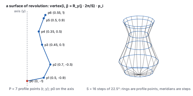
A sphere swept from a half-circle has a pole at each end and needs the fan at both; a cylinder or a vase whose profile stays off the axis needs none, and is open there. The guard in Section 5 is what keeps a forgotten pole from turning into NaN normals; the fan is what makes the guard unnecessary. The same machinery with a translation in place of the rotation is an extrusion (a cross-section pushed along a line), and with a general path and a frame carried along it is a sweep (a tube along a curve, see the curves chapter). All three are a cross-section times a sequence of rigid transforms, indexed as a grid.
9 · Surfaces from volumes: marching cubes
A third source of meshes is neither a formula nor a hand: a scalar field \(f(x, y, z)\) sampled on a grid, with the surface defined implicitly as the set where \(f = 0\). Medical scans (density), distance fields, fluid simulations, and the learned scenes of the learned-scenes chapter all produce their geometry this way, and the standard extractor is Lorensen and Cline’s marching cubes (1987).
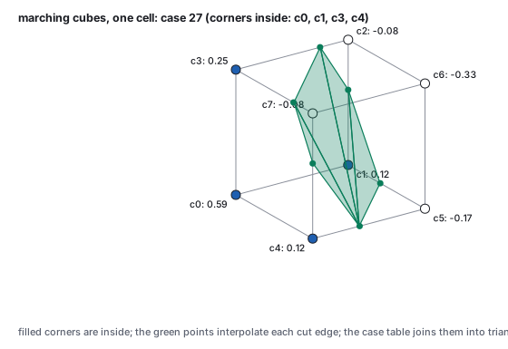
The mesh that comes out is manifold and closed wherever the field is, has vertices only on grid edges (so its resolution is the grid’s, and it aliases fine features exactly as a sampled image does), and needs the normal averaging of Section 5 or, better, the field’s own gradient as the normal. Dual contouring places one vertex inside each cell instead of one per edge and recovers sharp edges that marching cubes rounds off. Both produce more triangles than the shape needs, which is why the simplifier of the next section usually runs on their output.
10 · Simplification: the edge collapse and the quadric error
Scanned and sculpted meshes have far more triangles than any view needs. The Stanford bunny used in the course demos has 69,451 triangles at full resolution; at a distance where it covers a hundred pixels, nearly all of them are smaller than a pixel. Simplification removes triangles while keeping the shape, and one local operation does almost all of it.
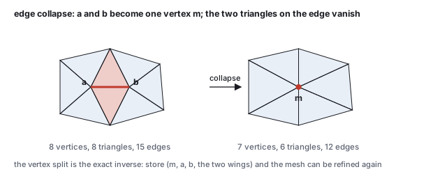
Which edge to collapse first, and where to put \(\mathbf{m}\)? Garland and Heckbert’s quadric error metric (1997) answers both with one number. Every vertex remembers the planes of the triangles around it. The cost of moving that vertex to a point \(\mathbf{x}\) is its summed squared distance to those planes: \[ Q(\mathbf{x}) = \sum_{\text{planes } (\mathbf{n}, d)} (\mathbf{n}\cdot\mathbf{x} + d)^2, \] with each plane stored as a unit normal \(\mathbf{n}\) and offset \(d = -\mathbf{n}\cdot\mathbf{p}\) for any point \(\mathbf{p}\) on it (the signed-distance form of the vectors chapter). The cost of collapsing \((\mathbf{a}, \mathbf{b})\) to \(\mathbf{m}\) is \(Q_a(\mathbf{m}) + Q_b(\mathbf{m})\): how far \(\mathbf{m}\) strays from every plane either endpoint used to lie on. Because \(Q\) is a quadratic in \(\mathbf{x}\), it is a \(4\times4\) symmetric matrix that adds when vertices merge, and its minimum is a \(3\times3\) linear solve. The algorithm puts every edge in a priority queue keyed by its minimal cost and collapses the cheapest edge until the target triangle count is reached.
| put \(\mathbf{m}\) at | \(Q(\mathbf{m})\) | why |
|---|---|---|
| \(\mathbf{v}_4 = (0, 0.4, 0)\) | 0.160 | on all six tilted planes; \(0.4^2\) from the floor plane of \(t_0\) |
| the midpoint \((0, 0.2, -0.75)\) | 0.404 | 0.2 from the floor, 0.19 to 0.39 from the far tilted planes |
| \(\mathbf{v}_1 = (0, 0, -1.5)\) | 1.457 | on \(t_0, t_1, t_2\); far below the four planes on the other side of the tent |
| the minimum, \((0, 0.338, 0)\) | 0.135 | the linear solve: slightly below the peak, trading a little floor error for less tilt error |
The quadric is a sum of squared plane distances, not a true distance to the surface, and it can be fooled (a vertex far from a plane along the plane’s own extension still reads as far); its virtues are that it is additive, that its minimum is closed-form, and that it costs one \(4\times4\) matrix per vertex. Whole families of simplifiers vary the cost (edge length, curvature, texture stretch, screen-space error) and the operation (vertex removal, vertex clustering, remeshing); the collapse with a queue is the one in the libraries, and it is what produced the bunny levels of the next section.
11 · Levels of detail and progressive meshes
An engine keeps several simplified versions of each model, its levels of detail (James Clark, 1976), and draws the coarsest one whose error is invisible at the current distance. The course’s bunny ladder was produced by greedy quadric collapse to four levels, and the error of each level against the full mesh was measured as the distance from the simplified surface to the original, in units of the model’s height:
| level | triangles | mean error | max error | median triangle aspect |
|---|---|---|---|---|
| L0 | 868 | \(3.2\times10^{-3}\) | \(1.5\times10^{-2}\) | 0.55 |
| L1 | 3,472 | \(1.0\times10^{-3}\) | \(6.3\times10^{-3}\) | 0.53 |
| L2 | 13,889 | \(2.7\times10^{-4}\) | \(1.9\times10^{-3}\) | 0.55 |
| L3 (full) | 69,451 | 0 | 0 | 0.60 |
Each level has a quarter of the triangles of the next and roughly three times its error: eighty times fewer triangles between L3 and L0 buys a maximum deviation of 1.5 % of the bunny’s height.
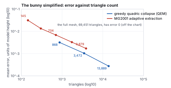
| level | max error | safe beyond \(d\) | pixels of error at \(d = 2\) |
|---|---|---|---|
| L2 (13,889) | 0.0019 | 1.7 | 0.8 |
| L1 (3,472) | 0.0064 | 5.5 | 2.8 |
| L0 (868) | 0.0154 | 13.4 | 6.7 |
Hoppe’s progressive mesh (1996) replaces the ladder with a continuum. Record every collapse of the simplification; the coarsest mesh plus the list of vertex splits, applied in reverse order, rebuilds every intermediate resolution exactly. The bunny’s stream stores a base of 1,368 vertices and 500 triangles followed by 34,579 split records; applying \(k\) of them gives a mesh of \(500 + 2k\) triangles for any \(k\), so the triangle count can track the distance continuously instead of in four steps, and the stream can be sent over a network coarse-first. The cost is that each split touches a few triangles, so changing resolution by a large amount is a loop of many small edits rather than one buffer swap.
Index order and the vertex cache
The GPU runs the vertex shader once per index, unless the vertex is in a small post-transform cache (16 to 32 entries) because a recent triangle used it. The cost of a mesh is therefore not \(3T\) shader runs but the average cache miss ratio (ACMR), misses per triangle, which depends only on the order of the index array. The grid at \(n = 10\) (121 vertices, 200 triangles) in row-major order has an ACMR of 1.10 with a 16-entry FIFO cache; the same triangles in a random order, 2.70; the lower bound, one miss per vertex, is \(121/200 = 0.605\), which a 32-entry cache reaches on the row-major order because a whole row of vertices then fits. Reordering triangles for locality (Forsyth’s 2006 heuristic, or the meshoptimizer library that produced the bunny levels) is a one-time offline pass that halves the vertex-shading cost of scanned meshes, and triangle strips were the earlier form of the same idea.
12 · Mesh files: OBJ and glTF
A mesh file stores the two arrays and, optionally, normals, texture coordinates and materials. Two formats cover most of what a graduate course meets. Wavefront OBJ (1990) is text, one vertex or face per line, with 1-based indices; the \(2\times2\) grid is
v -1.5 0 -1.5
v  0   0 -1.5
v  1.5 0 -1.5
v -1.5 0  0
v  0   0.4 0
v  1.5 0  0
v -1.5 0  1.5
v  0   0  1.5
v  1.5 0  1.5
f 1 4 2
f 2 4 5
f 2 5 3
f 3 5 6
f 4 7 5
f 5 7 8
f 5 8 6
f 6 8 9
Faces may have any number of sides (a quad is f 1 4 5 2), normals and coordinates
are separate lists joined by f 1/1/1 4/4/4 2/2/2 triples, and a vertex on a hard
edge or a seam is split at load time exactly as Section 5 describes, because OBJ indexes
position, normal and coordinate independently while the GPU indexes them together. The format is
readable and universal and has no binary form, no scene graph and no animation.
glTF 2.0 (Khronos, 2017) is the current interchange format for real-time work: a JSON document describing a scene graph (the nodes and local transforms of the scene-graphs chapter), meshes as primitives that point at typed binary buffers, PBR materials in the metallic-roughness form of the light-transport chapter, textures, skins and animation channels. The grid is one primitive with two accessors: positions, 9 vectors of 3 float32 (108 bytes), and indices, 24 uint16 (48 bytes), both in one binary buffer that the GPU can upload without parsing. The JSON says how to read them:
"meshes": [{ "primitives": [{ "attributes": { "POSITION": 0, "NORMAL": 1 }, "indices": 2, "mode": 4 }] }],
"accessors": [
  { "bufferView": 0, "componentType": 5126, "count": 9,  "type": "VEC3", "min": [-1.5,0,-1.5], "max": [1.5,0.4,1.5] },
  { "bufferView": 1, "componentType": 5126, "count": 9,  "type": "VEC3" },
  { "bufferView": 2, "componentType": 5123, "count": 24, "type": "SCALAR" } ]
mode 4 is a triangle list, 5126 is float32, 5123 is uint16, and the bounding box in
the position accessor is what a loader uses to frame the model. The course’s own
.mesh.bin files are a stripped version of the same idea: a 16-byte header with the
counts, then positions, normals, coordinates and indices as raw arrays. Whatever the format, the
loader ends with the two arrays of Section 1 and hands them to the GPU.