This chapter links to the course’s interactive demos and uses MathJax for its formulas. Read it through the course website (or download the file and open it in a browser); a Canvas inline preview will reach neither the demos nor the math. All chapters.

Rotation: Axis-Angle, Quaternions, Euler Angles

“How about sending me a fourth gimbal for Christmas?” Michael Collins, Apollo 11, when Houston warned of gimbal lock, 1969

A rotation keeps lengths and angles and fixes the origin, which makes it the best-behaved transform in graphics and, at the same time, the hardest to store well. A matrix applies it fast but drifts and cannot be blended; an axis and an angle say what it is; a quaternion stores it in four numbers that compose by multiplication and blend along a sphere; three Euler angles read nicely and lock; and “turn this direction onto that one” names the smallest rotation that does it. This chapter builds the four representations in that order, starting each in two dimensions where it can: what a rotation keeps, checked on a shape; the matrix as the landed axes; Rodrigues’ formula from the projection split of the vectors chapter, as the 2D rotation inside the plane across the axis; the quaternion as the 3D descendant of the unit complex number, with its sandwich worked on a point and the half angle taken apart one factor at a time; composition, blending and Euler angles. The Appendix recovers an axis and angle from a matrix, steps small rotations, converts a quaternion to a matrix and back, extracts Euler angles at the lock, and measures the drift with real single-precision arithmetic. One axis and angle, \((0, 1, 0)\) at \(30^\circ\), runs through the worked examples and the live demo.

Contents
  1. What a rotation preserves
  2. The rotation matrix: columns are where the axes land
  3. Axis-angle: Rodrigues’ formula
  4. Quaternions
  5. Composition and interpolation
  6. Euler angles and gimbal lock
  7. Choosing a representation
  8. In code
  9. Exercises
Appendix: the log map, small angles and angular velocity, quaternion to matrix and back, extracting Euler angles, drift.

1 · What a rotation preserves

Definition (rotation) A rotation is a linear map \(R\) that preserves the dot product, \((R\mathbf{u})\cdot(R\mathbf{v}) = \mathbf{u}\cdot\mathbf{v}\), and preserves handedness. (Linear: it sends sums to sums and multiples to multiples, \(R(a\mathbf{u} + b\mathbf{v}) = aR\mathbf{u} + bR\mathbf{v}\).) Preserving dot products preserves lengths and angles; linearity fixes the origin. In matrix terms, \(R^{\mathsf T}R = I\) and \(\det R = +1\): the columns of \(R\) are unit and mutually perpendicular. (With \(\det R = -1\) the map is a reflection, which also keeps lengths and angles but turns a right hand into a left one.)
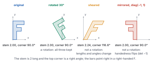
Four panels: an F shape; the F rotated by 30 degrees, stem 2 and top corner 90 degrees as before; the F sheared, stem 2.24 and corner 116.6 degrees; the F mirrored, stem 2 and corner 90 degrees but turned over, its bars pointing left.
What a rotation keeps, measured on an F: the stem’s length, the top corner’s angle and the side the bars point to. A shear changes the first two; a mirror keeps them and turns the shape over (determinant \(-1\)). Computed with the 2D matrices named in the panels.

Because a rotation is linear and fixes the origin, it is completely determined by where it sends the three basis vectors. That one fact makes rotation matrices readable, which is the next section.

1.1 The three properties, and why they follow from one

Orthogonal matrices The transpose \(R^{\mathsf T}\) is \(R\) with its rows written as columns, so entry \((i, j)\) of \(R^{\mathsf T}R\) is column \(i\) of \(R\) dotted with column \(j\). If \(R^{\mathsf T}R = I\) then: (i) \(R^{-1} = R^{\mathsf T}\), so the inverse costs nothing; (ii) the columns are orthonormal (entry \((i, j)\) of \(R^{\mathsf T}R\) is column \(i\) dotted with column \(j\)), and so are the rows; (iii) \(\det R = \pm1\), since \(\det(R^{\mathsf T}R) = (\det R)^2 = 1\). The sign of the determinant, which is the scalar triple product of the columns (the vectors chapter, Section 3.2), separates rotations (\(+1\)) from reflections (\(-1\)).
Worked example (checking \(R_y(30^\circ)\)) The library’s matrix has rows \((0.866, 0, 0.5)\), \((0, 1, 0)\), \((-0.5, 0, 0.866)\). Column 0 dotted with itself: \(0.866^2 + 0.5^2 = 0.75 + 0.25 = 1\); column 0 with column 2: \(0.866\cdot0.5 + 0 - 0.5\cdot0.866 = 0\); the full product \(R^{\mathsf T}R\) is the identity to \(10^{-6}\) in every entry. The determinant is \(0.866\cdot0.866 - 0.5\cdot(-0.5) = 1\). And the transpose undoes the rotation: \(R^{\mathsf T}(1.016, 0.6, -0.24) = (1, 0.6, 0.3)\), the vector Section 3 started from. Nine numbers, six constraints (three unit lengths, three right angles), three degrees of freedom left: three numbers can still be chosen freely, two to aim the new \(x\) axis and one to twist the new \(y\) axis about it, and the new \(z\) axis is then forced to be their cross product.

1.2 Reflections, and why two of them are a rotation
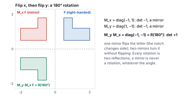
A blue F-shaped polygon in the first quadrant, its red mirror image across the y axis in the second quadrant, and the green image of that reflected again across the x axis in the third quadrant, which is the original turned by 180 degrees; the three matrices and their determinants are listed.
\(\mathrm{diag}(-1, 1)\) and \(\mathrm{diag}(1, -1)\) each have determinant \(-1\) and each flips the shape; their product \(\mathrm{diag}(-1, -1)\) has determinant \(+1\) and is a half turn. The notch on the F is the handedness witness.
Worked example (a mirror is not a rotation) The mirror \(M_x = \mathrm{diag}(-1, 1, 1)\) has orthonormal columns and \(\det M_x = -1\). It sends \(\hat{\mathbf{x}}\times\hat{\mathbf{y}} = \hat{\mathbf{z}}\) to \((M_x\hat{\mathbf{x}})\times(M_x\hat{\mathbf{y}}) = (-\hat{\mathbf{x}})\times\hat{\mathbf{y}} = -\hat{\mathbf{z}}\), while it sends \(\hat{\mathbf{z}}\) itself to \(+\hat{\mathbf{z}}\): the cross product of the images is not the image of the cross product, which is what “handedness flipped” means in arithmetic. Two mirrors compose to \(M_y M_x = \mathrm{diag}(-1, -1, 1)\), determinant \(+1\), which is \(R_z(180^\circ)\). Every rotation is a product of two reflections, and no product of an odd number of reflections is a rotation. A model imported with one negative scale factor is in the second class, which the affine chapter returns to. (\(\mathrm{diag}(a, b, c)\) is the matrix with \(a, b, c\) on its diagonal and zeros elsewhere: it scales the three axes.)
See it live One rotation, five definitions, in its columns mode: aim the new \(x\) axis (two sliders) and twist the new \(y\) axis about it (one slider); the new \(z\) axis is forced to be \(x' \times y'\), which is the three degrees of freedom in your hands. The mirror switch sets \(z' = -(x' \times y')\): the determinant reads \(-1\) and the cube turns into its mirror image.

2 · The rotation matrix: columns are where the axes land

In two dimensions, a point at radius \(r\) and angle \(\varphi\) is \((r\cos\varphi, r\sin\varphi)\); rotating it by \(\theta\) gives \((r\cos(\varphi + \theta), r\sin(\varphi + \theta))\). Expand with the angle-addition formulas and regroup in terms of \(x = r\cos\varphi\), \(y = r\sin\varphi\):

\[ \begin{pmatrix} x' \\ y' \end{pmatrix} = \begin{pmatrix} \cos\theta & -\sin\theta \\ \sin\theta & \cos\theta \end{pmatrix} \begin{pmatrix} x \\ y \end{pmatrix}. \]
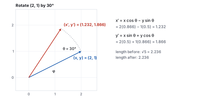
The point (2,1) rotated by 30 degrees to (1.232, 1.866), with the arc it travels and the two formulas evaluated beside it; the length 2.236 is unchanged.
The one derivation everything else lifts from. Feed the matrix \((1, 0)\) and you get its first column, \((\cos\theta, \sin\theta)\): where the \(x\) axis lands. Feed it \((0, 1)\) and you get the second column: where the \(y\) axis lands.
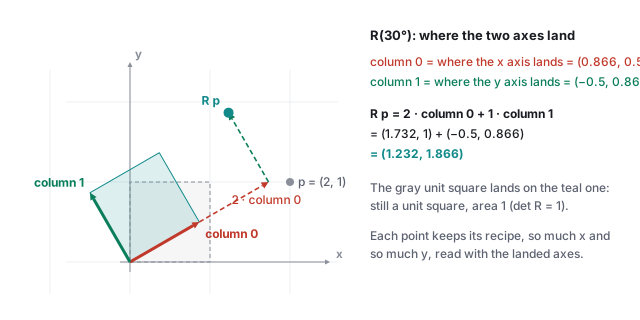
The column reading A matrix times a vector is a mix of the matrix’s columns: \(M\mathbf{v} = v_x\,(\text{column }0) + v_y\,(\text{column }1) + v_z\,(\text{column }2)\). Feed it a basis vector and only one column survives, so for any linear map, column \(j\) of the matrix is the image of the \(j\)-th basis vector. A rotation matrix is therefore its rotated basis vectors, stacked as columns. You can read where any axis goes without multiplying anything. Its rows are the same statement for the inverse: row \(i\) is where the \(i\)-th axis came from.
The x and y axes turned by 30 degrees land at (0.866, 0.5) and (-0.5, 0.866), the two columns; the point (2, 1) lands at twice the first column plus once the second, (1.232, 1.866); the unit square lands on a unit square.
The column reading in 2D. The point \((2, 1)\) is two steps along \(x\) and one along \(y\); after the turn it is two steps along the landed \(x\) axis and one along the landed \(y\) axis: \(2\,(0.866, 0.5) + (-0.5, 0.866) = (1.232, 1.866)\), the answer the formula gave. The unit square lands on a unit square, so the area, which is the determinant, stays 1.

Rotation about the \(y\) axis leaves \(y\) alone and spins the \(x\)–\(z\) plane, so the 2D block drops into the \(x, z\) slots:

\[ R_y(\theta) = \begin{pmatrix} \cos\theta & 0 & \sin\theta \\ 0 & 1 & 0 \\ -\sin\theta & 0 & \cos\theta \end{pmatrix}, \qquad R_y(30^\circ) = \begin{pmatrix} 0.866 & 0 & 0.5 \\ 0 & 1 & 0 \\ -0.5 & 0 & 0.866 \end{pmatrix}. \]

Watch the sign pattern: for \(R_y\) the \(+\sin\) sits top-right, the opposite of the textbook \(R_z\). Look down from above, with \(y\) pointing at you, \(z\) to the right and \(x\) up: the turn about \(y\) is the ordinary counter-clockwise 2D rotation with \(z\) in the role of \(x\) and \(x\) in the role of \(y\), so \(z\) tips toward \(x\) and \(x\) tips toward \(-z\). Column 0 says so: \((\cos\theta, 0, -\sin\theta)\).
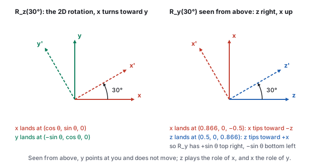
Left: the 2D rotation by 30 degrees turning x toward y. Right: the rotation about y seen from above, z to the right and x up, the same counter-clockwise turn: x lands at (0.866, 0, -0.5) and z at (0.5, 0, 0.866).
\(R_y\) is the 2D rotation of the \(z\)–\(x\) plane. Seen from above, the same counter-clockwise turn sends \(x\) to \((0.866, 0, -0.5)\) and \(z\) to \((0.5, 0, 0.866)\), columns 0 and 2 of the library’s \(R_y(30^\circ)\).

The three axis rotations for reference, all counter-clockwise when looking down the axis toward the origin:

\[ R_x(\theta) = \begin{pmatrix} 1 & 0 & 0 \\ 0 & \cos\theta & -\sin\theta \\ 0 & \sin\theta & \cos\theta \end{pmatrix}, \quad R_z(\theta) = \begin{pmatrix} \cos\theta & -\sin\theta & 0 \\ \sin\theta & \cos\theta & 0 \\ 0 & 0 & 1 \end{pmatrix}. \]
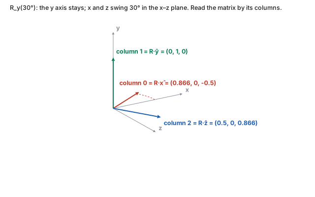
A 3D diagram of the three columns of R_y(30 degrees) drawn as arrows from the origin: column 0 at (0.866, 0, -0.5), column 1 still (0,1,0), column 2 at (0.5, 0, 0.866), each labeled with its coordinates.
\(R_y(30^\circ)\) read by its columns, computed by the course library. At \(90^\circ\) column 0 is \((0, 0, -1)\): the old \(x\) axis points down \(-z\). Predict any axis’s destination by reading a column.

3 · Axis-angle: Rodrigues’ formula

A rotation can be about any unit axis \(\hat{\mathbf{n}}\) by any angle \(\theta\). That pair is the most human representation (“turn 40 degrees about this stick”), and applying it to a vector needs only the projection split and one cross product.

  1. Split \(\mathbf{v}\) into the part along the axis, which a rotation about that axis cannot move, and the part across it: \(\mathbf{v}_\parallel = (\mathbf{v}\cdot\hat{\mathbf{n}})\hat{\mathbf{n}}\), \(\mathbf{v}_\perp = \mathbf{v} - \mathbf{v}_\parallel\).
  2. Build the second axis of the rotation plane: \(\mathbf{w} = \hat{\mathbf{n}}\times\mathbf{v}\) is perpendicular to both \(\hat{\mathbf{n}}\) and \(\mathbf{v}_\perp\) and has the same length as \(\mathbf{v}_\perp\), since \(\|\hat{\mathbf{n}}\times\mathbf{v}\| = \|\mathbf{v}\|\sin\angle(\hat{\mathbf{n}},\mathbf{v}) = \|\mathbf{v}_\perp\|\).
  3. Turn inside the plane, a 2D rotation with \(\mathbf{v}_\perp\) and \(\mathbf{w}\) as the two axes: \(\mathbf{v}_\perp' = \cos\theta\,\mathbf{v}_\perp + \sin\theta\,\mathbf{w}\).
  4. Add the frozen part back and substitute.
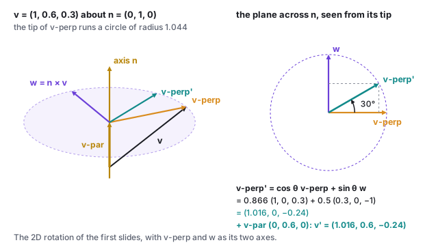
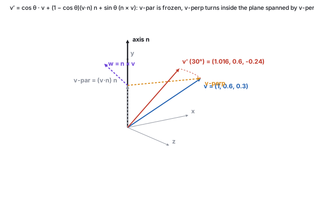
Left: v = (1, 0.6, 0.3), its frozen part along the axis n = (0, 1, 0), its turning part v-perp and w = n x v on the circle of radius 1.044 across the axis. Right: that plane seen from the tip of n, v-perp to the right and w up, v-perp turned by 30 degrees to cos 30 v-perp + sin 30 w.
Step 3 is the 2D rotation. Seen from the tip of \(\hat{\mathbf{n}}\), the plane across the axis is an ordinary plane with \(\mathbf{v}_\perp\) and \(\mathbf{w}\) as its two axes, both of length \(1.044\); turning by \(30^\circ\) gives \(0.866\,\mathbf{v}_\perp + 0.5\,\mathbf{w} = (1.016, 0, -0.24)\), and adding \(\mathbf{v}_\parallel\) back gives \(\mathbf{v}' = (1.016, 0.6, -0.24)\).
Rodrigues’ rotation formula \[ \mathbf{v}' \;=\; \cos\theta\,\mathbf{v} \;+\; (1 - \cos\theta)\,(\mathbf{v}\cdot\hat{\mathbf{n}})\,\hat{\mathbf{n}} \;+\; \sin\theta\,(\hat{\mathbf{n}}\times\mathbf{v}) . \] Every term is a dot, a cross, or a scale. Apply it to \(\hat{\mathbf{x}}, \hat{\mathbf{y}}, \hat{\mathbf{z}}\) and the three results are the columns of the rotation matrix.
A 3D diagram: the axis n pointing up, a vector v = (1, 0.6, 0.3), its frozen part along the axis, its perpendicular part, the cross product w = n x v, and the rotated vector v-prime = (1.016, 0.6, -0.24) after a 30 degree turn, with the arc it sweeps.
The construction on \(\mathbf{v} = (1, 0.6, 0.3)\) about \(\hat{\mathbf{n}} = (0,1,0)\): \(\mathbf{v}_\parallel = (0, 0.6, 0)\), \(\mathbf{v}_\perp = (1, 0, 0.3)\), \(\mathbf{w} = (0.3, 0, -1)\), both of length \(1.044\). The rotated vector keeps its \(y\) component and swings the rest.
Worked example (Rodrigues on one vector, and against the matrix) \(\hat{\mathbf{n}} = (0,1,0)\), \(\theta = 30^\circ\), \(\mathbf{v} = (1, 0.6, 0.3)\), so \(\mathbf{v}\cdot\hat{\mathbf{n}} = 0.6\) and \(\hat{\mathbf{n}}\times\mathbf{v} = (1\cdot0.3 - 0\cdot0.6,\; 0\cdot1 - 0\cdot0.3,\; 0\cdot0.6 - 1\cdot1) = (0.3, 0, -1)\). \[ \begin{aligned} \mathbf{v}' &= 0.866\,(1, 0.6, 0.3) + 0.134\cdot0.6\,(0,1,0) + 0.5\,(0.3, 0, -1) \\ &= (0.866 + 0.15,\; 0.520 + 0.080,\; 0.260 - 0.5) \\ &= (1.016, 0.6, -0.240). \end{aligned} \] The library’s matrix \(R_y(30^\circ)\) applied to the same \(\mathbf{v}\) gives \((1.016, 0.6, -0.240)\): the formula and the matrix are one object reached two ways.
Worked example (build \(R_y(30^\circ)\) column by column)
basis vector\(\mathbf{v}\cdot\hat{\mathbf{n}}\)\(\hat{\mathbf{n}}\times\mathbf{v}\)\(\mathbf{v}'\)
\(\hat{\mathbf{x}} = (1,0,0)\)0\((0, 0, -1)\)\(0.866\,(1,0,0) + 0.5\,(0,0,-1) = (0.866, 0, -0.5)\)
\(\hat{\mathbf{y}} = (0,1,0)\)1\((0,0,0)\)\((0, 1, 0)\), unchanged
\(\hat{\mathbf{z}} = (0,0,1)\)0\((1, 0, 0)\)\(0.866\,(0,0,1) + 0.5\,(1,0,0) = (0.5, 0, 0.866)\)
The three rows are the three columns of the matrix in Section 2, digit for digit, and they are what the demo’s \(R\) panel shows.
See it live Axis-angle rotation: a cube spins about a draggable axis; the panel prints the matrix and the quaternion, both from the course’s own code. Drag the angle and watch column 0 trace \((\cos\theta, 0, -\sin\theta)\). The Rodrigues construction layer draws this section’s vectors for \(\mathbf{v} = (1, 0.6, 0.3)\): the frozen part \(\mathbf{v}_\parallel\), the turning part \(\mathbf{v}_\perp\), \(\mathbf{w} = \hat{\mathbf{n}}\times\mathbf{v}\), and \(\mathbf{v}'\) sweeping its circle of radius \(1.044\) at height \(0.6\).

3.1 Rodrigues as a matrix

The cross product with a fixed vector is a linear map, so it has a matrix. For a unit axis \(\hat{\mathbf{n}} = (n_x, n_y, n_z)\), \[ K = \begin{pmatrix} 0 & -n_z & n_y \\ n_z & 0 & -n_x \\ -n_y & n_x & 0 \end{pmatrix}, \qquad K\mathbf{v} = \hat{\mathbf{n}}\times\mathbf{v}, \] and \(K\) is skew-symmetric, \(K^{\mathsf T} = -K\). Two applications give \(K^2\mathbf{v} = \hat{\mathbf{n}}\times(\hat{\mathbf{n}}\times\mathbf{v}) = (\mathbf{v}\cdot\hat{\mathbf{n}})\hat{\mathbf{n}} - \mathbf{v}\), which is minus the perpendicular part of \(\mathbf{v}\). Substituting both into Rodrigues’ formula turns it into a matrix identity:

The rotation matrix about any axis \[ R(\hat{\mathbf{n}}, \theta) = I + \sin\theta\,K + (1 - \cos\theta)\,K^2 . \] This is what the library’s axisAngleMatrix evaluates. Set \(\hat{\mathbf{n}} = \hat{\mathbf{y}}\) and the three \(R_y\) entries of Section 2 fall out of \(K\) and \(K^2\).
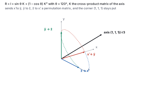
A 3D diagram with the axis (1,1,1)/sqrt(3) drawn as a heavy black arrow and the three basis vectors in red, green and blue, each with a dashed arc showing its path under a 120 degree turn: x goes to y, y to z, z to x.
\(R\big((1,1,1)/\sqrt3,\; 120^\circ\big)\) is the permutation that cycles the axes. Each basis vector travels a third of a circle about the diagonal and lands on the next one; the corner \((1, 1, 1)\) of the cube is on the axis and does not move.
Worked example (the diagonal axis at \(120^\circ\)) \(\hat{\mathbf{n}} = (1, 1, 1)/\sqrt3 = (0.577, 0.577, 0.577)\), so every off-diagonal entry of \(K\) is \(\pm0.577\), and \(K^2\) has \(-0.667\) on its diagonal and \(0.333\) elsewhere. With \(\sin 120^\circ = 0.866\) and \(1 - \cos 120^\circ = 1.5\), the entry \((1, 0)\) is \(0 + 0.866\cdot0.577 + 1.5\cdot0.333 = 0.5 + 0.5 = 1\) and the entry \((0, 0)\) is \(1 + 0 + 1.5\cdot(-0.667) = 0\). Finishing the nine entries gives \[ R = \begin{pmatrix} 0 & 0 & 1 \\ 1 & 0 & 0 \\ 0 & 1 & 0 \end{pmatrix}, \] exactly the library’s \(R\) for that axis and angle. Its columns say \(\hat{\mathbf{x}}\mapsto\hat{\mathbf{y}}\), \(\hat{\mathbf{y}}\mapsto\hat{\mathbf{z}}\), \(\hat{\mathbf{z}}\mapsto\hat{\mathbf{x}}\), and \(R(1,1,1) = (1,1,1)\): a point on the axis is fixed, as it must be. Three of these turns are the identity.

4 · Quaternions

Why not store the matrix? Nine numbers with six hidden constraints, for three degrees of freedom. Composing matrices in floating point erodes the constraints and shapes begin to shear (Appendix A.5 measures it); averaging two rotation matrices is not a rotation, so orientations cannot be blended. A quaternion has four numbers, one constraint, composes by multiplication, and blends along a sphere.
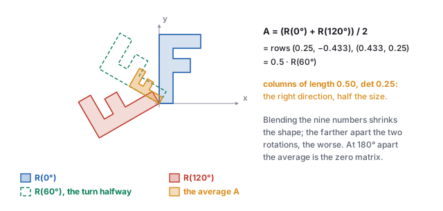
An F shape under the identity, under a 120 degree rotation, under the 60 degree rotation halfway between, and under the entry-by-entry average of the first two matrices, which is half the size of the 60 degree one.
Averaging matrices, in 2D. \(\tfrac12\big(R(0^\circ) + R(120^\circ)\big)\) has rows \((0.25, -0.433)\) and \((0.433, 0.25)\): it is \(0.5\,R(60^\circ)\), the turn halfway but at half the size (columns of length \(0.5\), determinant \(0.25\)). At \(180^\circ\) apart the average is the zero matrix.

4.0 What a quaternion is

A complex number \(a + b\,i\) with \(i^2 = -1\) is a point of the plane, and multiplying by the unit complex number \(\cos\theta + i\sin\theta\) turns the plane by \(\theta\): \((x + y\,i)(\cos\theta + i\sin\theta) = (x\cos\theta - y\sin\theta) + (x\sin\theta + y\cos\theta)\,i\), the two rows of the 2D matrix of Section 2. For the point \((2, 1)\) and \(30^\circ\), \((2 + i)(0.866 + 0.5\,i) = 1.232 + 1.866\,i\), the same numbers. Two turns compose by multiplying, the angles add, and the order does not matter; in three dimensions it does (Section 5), so the three-dimensional version needs a product whose order matters.
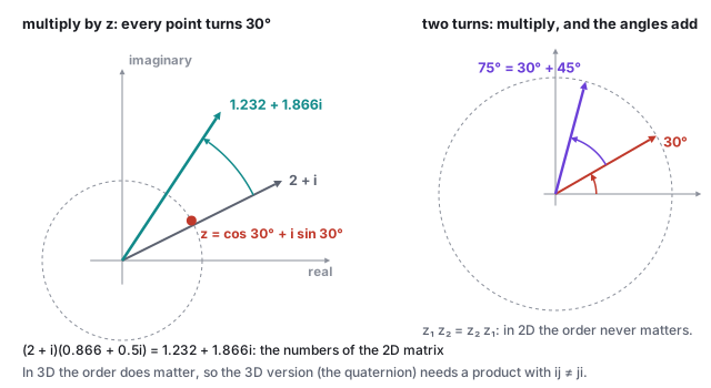
Left: 2 + i multiplied by cos 30 + i sin 30 turns 30 degrees to 1.232 + 1.866i. Right: on the unit circle, the turns of 30 and 45 degrees multiply to the turn of 75 degrees.
In 2D a rotation is one multiplication by a unit complex number, and turns compose by adding angles, in either order. Computed by complex multiplication.

William Rowan Hamilton spent years looking for the three-dimensional version and found, on 16 October 1843, that it needs three imaginary units. A quaternion is \(w + x\,i + y\,j + z\,k\), multiplied by the rule he carved into Broom Bridge in Dublin,

\[ i^2 = j^2 = k^2 = ijk = -1, \qquad\text{so}\qquad ij = k,\; jk = i,\; ki = j, \qquad ji = -k,\; kj = -i,\; ik = -j . \]

\(w\) is the scalar part and \((x, y, z)\) the vector part; the words entered mathematics here. Writing a quaternion as (vector part, scalar part) and expanding a product term by term with these rules gives

\[ (\mathbf{v}, w)\,(\mathbf{u}, s) = \big(w\,\mathbf{u} + s\,\mathbf{v} + \mathbf{v}\times\mathbf{u},\;\; ws - \mathbf{v}\cdot\mathbf{u}\big), \]

a dot, a cross and two scalings. The cross product is why the product does not commute, and rotations do not commute either.

Definition (unit quaternion of a rotation) For axis \(\hat{\mathbf{n}}\) and angle \(\theta\), \[ q = \big(\sin\tfrac{\theta}{2}\,\hat{\mathbf{n}},\; \cos\tfrac{\theta}{2}\big) = (x, y, z, w), \] three “vector” components and one scalar \(w\), in the storage order of three.js and Unity. It has unit length: \(x^2 + y^2 + z^2 + w^2 = \sin^2\tfrac\theta2 + \cos^2\tfrac\theta2 = 1\). The identity is \((0, 0, 0, 1)\). The inverse of a unit quaternion is its conjugate, the vector part negated, \(q^{-1} = (-x, -y, -z, w)\): same axis, opposite angle.
Worked example (the quaternion for \(R_y(30^\circ)\)) Half angle \(15^\circ\): \(\sin 15^\circ = 0.259\), \(\cos 15^\circ = 0.966\), so \(q = (0, 0.259, 0, 0.966)\). Only the \(y\) component is nonzero because the axis is \(y\). Unit length: \(0.259^2 + 0.966^2 = 0.067 + 0.933 = 1.000\). This is the demo panel’s \(q\) row.

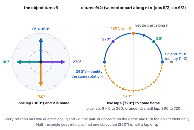
The half angle is the one surprise. It comes from how a quaternion rotates a point: write the point as the quaternion \((\mathbf{p}, 0)\) and multiply on both sides, a sandwich, \(p' = q\,p\,q^{-1}\). Split \(\mathbf{p}\) as in Section 3. On the part across the axis, \(\hat{\mathbf{n}}\cdot\mathbf{p} = 0\), so the product rule above gives \(q\,(\mathbf{p}, 0) = (\cos\tfrac\theta2\,\mathbf{p} + \sin\tfrac\theta2\,\hat{\mathbf{n}}\times\mathbf{p},\; 0)\): the left factor turns it by \(\theta/2\), and the right factor \(q^{-1}\) turns it by another \(\theta/2\). On the part along the axis, the left factor tilts it into the fourth (\(w\)) component and the right factor tilts it back, leaving it unchanged. So the point turns by \(\theta\) while \(q\) itself has turned only \(\theta/2\). A one-sided product \(q\,p\) would turn the across part by half the angle and smear the along part into \(w\); the sandwich is what makes the halves add.
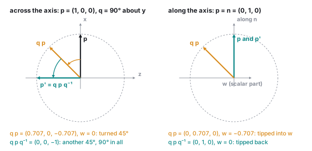
Left, seen from above: p = (1, 0, 0), q p turned 45 degrees to (0.707, 0, -0.707), and q p q-inverse turned 90 degrees to (0, 0, -1). Right: p along the axis tips into the scalar part w after q p, to (0, 0.707, 0) with w = -0.707, and back to (0, 1, 0) after the right factor.
The sandwich one factor at a time, for \(q\) = \(90^\circ\) about \(y\), computed with the library’s quaternion product. Across the axis each factor turns \(\mathbf{p}\) by \(45^\circ\); along the axis the left factor tips \(\mathbf{p}\) into \(w\) and the right factor tips it back.
Left: an object turned by theta at 0, 90, 180, 270 and 360 degrees, back home at 360. Right: the quaternion's point (cos theta/2, sin theta/2) on a unit circle, reaching (0, 1) at theta = 180 and (-1, 0), minus the identity, at theta = 360, and home again only at 720.
The object needs one lap, \(360^\circ\), to come home; \(q\) needs two. At \(\theta = 360^\circ\) the object is back where it started and \(q = (0, 0, 0, -1)\), minus the identity: every rotation has two quaternions (Section 4.1).
See it live The axis-angle demo’s half angle layer shows two dials: the cube’s turn \(\theta\) and \(q\)’s point \((\cos\tfrac\theta2, \sin\tfrac\theta2)\). Drag to \(180^\circ\) (\(w = 0\)) and to \(360^\circ\) (the cube is home, \(q = (0, 0, 0, -1)\)).

Expanded into vector operations (with \(\mathbf{q}_v = (x, y, z)\)) the sandwich needs no trigonometry at all:

\[ \mathbf{p}' \;=\; \mathbf{p} \;+\; 2w\,(\mathbf{q}_v\times\mathbf{p}) \;+\; 2\,\mathbf{q}_v\times(\mathbf{q}_v\times\mathbf{p}) . \]
Worked example (the sandwich on one point) Rotate \(\mathbf{p} = (1,0,0)\) by \(90^\circ\) about \(y\): \(q = (0, 0.707, 0, 0.707)\), \(\mathbf{q}_v = (0, 0.707, 0)\), \(w = 0.707\).
\(\mathbf{q}_v\times\mathbf{p}\)\((0, 0.707, 0)\times(1, 0, 0) = (0.707\cdot0 - 0,\; 0 - 0,\; 0 - 0.707\cdot1) = (0, 0, -0.707)\)
\(2w\,(\mathbf{q}_v\times\mathbf{p})\)\(1.414\,(0, 0, -0.707) = (0, 0, -1)\)
\(\mathbf{q}_v\times(\mathbf{q}_v\times\mathbf{p})\)\((0, 0.707, 0)\times(0, 0, -0.707) = (0.707\cdot(-0.707) - 0,\; 0,\; 0) = (-0.5, 0, 0)\)
\(2\,\mathbf{q}_v\times(\cdots)\)\((-1, 0, 0)\)
sum\((1,0,0) + (0,0,-1) + (-1,0,0) = (0, 0, -1)\)
\(R_y(90^\circ)\) sends \((1,0,0)\) to \((0,0,-1)\) (its column 0). The quaternion and the matrix agree.
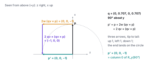
Seen from above, z to the right and x up: p = (1, 0, 0) up, the term 2w(qv x p) = (0, 0, -1) to the left, the term 2 qv x (qv x p) = (-1, 0, 0) down, ending at p' = (0, 0, -1) on the unit circle.
The worked example as three arrows, tip to tail, seen from above: up 1, left 1, down 1, and the end lands on the circle at \((0, 0, -1)\).

4.1 The double cover

\(q\) and \(-q\) give the same rotation: the sandwich \((-q)\,p\,(-q)^{-1}\) uses the quaternion twice, and the two signs cancel. So \((0, -0.259, 0, -0.966)\) is also \(R_y(30^\circ)\); it is the quaternion of \(R_y(390^\circ)\), a full extra turn, and \(\sin 195^\circ, \cos 195^\circ\) are exactly those numbers. Every rotation has two quaternions, antipodal on the unit sphere. This matters in exactly one place, interpolation: the arc from \(q_1\) to \(q_2\) and the arc from \(q_1\) to \(-q_2\) reach the same orientation, but one is short and the other goes the long way round. Section 5 tests the sign of \(q_1\cdot q_2\) for that reason. The name for the two-to-one relation is the double cover: the unit quaternions cover the rotations twice.
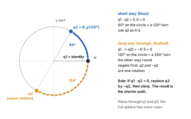
The circle through the identity and q2: q2 sits 60 degrees from the identity, minus q2 sits 120 degrees away; the short arc is a 120 degree turn and the long arc a 240 degree turn the other way.
\(q_2\) and \(-q_2\) are the same orientation, \(R_y(120^\circ)\). From the identity, the arc to \(q_2\) (\(q_1\cdot q_2 = 0.5 > 0\)) is a \(120^\circ\) turn; the arc to \(-q_2\) (\(q_1\cdot(-q_2) = -0.5\)) is a \(240^\circ\) turn the other way.

5 · Composition and interpolation

Do rotation \(q_1\), then \(q_2\): multiply, \(q = q_2\,q_1\), with the one nearest the point applied first, the same right-to-left reading as matrices. The product is

\[ \begin{aligned} (q_1 q_2)_x &= \phantom{-}x_1 w_2 + y_1 z_2 - z_1 y_2 + w_1 x_2, \\ (q_1 q_2)_y &= -x_1 z_2 + y_1 w_2 + z_1 x_2 + w_1 y_2, \\ (q_1 q_2)_z &= \phantom{-}x_1 y_2 - y_1 x_2 + z_1 w_2 + w_1 z_2, \\ (q_1 q_2)_w &= -x_1 x_2 - y_1 y_2 - z_1 z_2 + w_1 w_2, \end{aligned} \]

sixteen multiplies against a 3×3 product’s twenty-seven, and the result stays a rotation after a single renormalization. In vector form the same product is \(\mathbf{q}_v = w_1\mathbf{q}_{2v} + w_2\mathbf{q}_{1v} + \mathbf{q}_{1v}\times\mathbf{q}_{2v}\), \(w = w_1 w_2 - \mathbf{q}_{1v}\cdot\mathbf{q}_{2v}\): a cross product sits inside it, which is why it is not commutative, exactly as rotations are not. Pitch then yaw is not yaw then pitch.
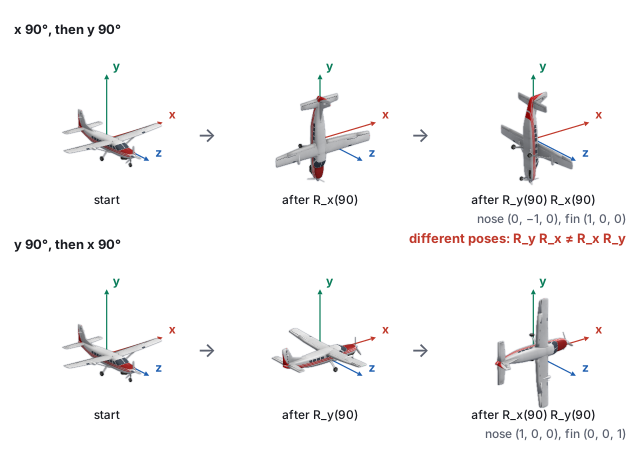
Worked example (compose two rotations, check against the matrices) \(R_y(30^\circ)\) first, then \(R_x(30^\circ)\): \(q_y = (0, 0.259, 0, 0.966)\), \(q_x = (0.259, 0, 0, 0.966)\), and \(q = q_x\,q_y\): \[ q = (0.25,\; 0.25,\; 0.067,\; 0.933), \qquad |q|^2 = 1.000 . \] Applied to \((1, 2, 3)\) by the sandwich: \((2.366, 0.683, 2.817)\). The matrix product \(R_x(30^\circ)\,R_y(30^\circ)\) applied to the same point: \((2.366, 0.683, 2.817)\). The composite is itself one rotation: reading \(q\) back, its angle is \(2\arccos 0.933 = 42.2^\circ\) about the axis \((0.695, 0.695, 0.186)\), a single turn about a tilted axis that no one specified. Two rotations about two axes are always one rotation about a third, and Appendix A.1 reads the same axis and angle out of the matrix. The other order, \(q_y\,q_x = (0.25, 0.25, -0.067, 0.933)\), differs only in the sign of the cross-product term, and its pose is \(15.4^\circ\) away.
Two rows of three poses of a Cessna 208 model: x 90 degrees then y 90 degrees, and y 90 degrees then x 90 degrees; the final poses differ.
Order matters: the same two quarter turns in the two orders, computed with the library’s matrices. Each final pose is itself one \(120^\circ\) turn, about two different cube diagonals.
See it live Composing rotations: two copies of an object, “A then B” and “B then A”, with the single equivalent axis of each drawn in gold. Play animates the two sequences; set both angles to \(90^\circ\), then put both turns on the same axis and watch the two orders agree.

5.1 From one direction to another

A fifth way to name a rotation: “turn this direction onto that one”, as when a head turns toward a target. For unit vectors \(\mathbf{a}\) and \(\mathbf{b}\), the smallest such rotation has axis \(\mathbf{a}\times\mathbf{b}\) and angle \(\arccos(\mathbf{a}\cdot\mathbf{b})\), and its quaternion needs no trigonometry: since \(1 + \mathbf{a}\cdot\mathbf{b} = 1 + \cos\theta = 2\cos^2\tfrac\theta2\) and \(\|\mathbf{a}\times\mathbf{b}\| = \sin\theta = 2\sin\tfrac\theta2\cos\tfrac\theta2\), both carry the factor \(2\cos\tfrac\theta2\), and

\[ q = \mathrm{normalize}\big(\mathbf{a}\times\mathbf{b},\; 1 + \mathbf{a}\cdot\mathbf{b}\big) \]

is exactly \((\sin\tfrac\theta2\,\hat{\mathbf{n}}, \cos\tfrac\theta2)\). Unity’s Quaternion.FromToRotation and three.js’s setFromUnitVectors compute it. It names one rotation among many: any extra twist about \(\mathbf{b}\) also sends \(\mathbf{a}\) onto \(\mathbf{b}\), and this one has none.
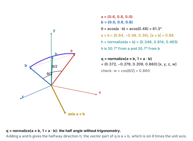
Unit vectors a and b from the origin, the 61.3 degree arc from a to b, the rotation axis a cross b, and the halfway direction normalize(a + b) at half the angle from each.
The shortest arc from \(\mathbf{a} = (0.6, 0.8, 0)\) to \(\mathbf{b} = (0, 0.6, 0.8)\): axis along \(\mathbf{a}\times\mathbf{b}\), angle \(61.3^\circ\); the halfway direction \(\mathrm{normalize}(\mathbf{a} + \mathbf{b})\) sits at \(\theta/2\) from each.
Worked example (the shortest arc) \(\mathbf{a} = (0.6, 0.8, 0)\), \(\mathbf{b} = (0, 0.6, 0.8)\): \(\mathbf{a}\cdot\mathbf{b} = 0.48\), \(\mathbf{a}\times\mathbf{b} = (0.8\cdot0.8 - 0,\; 0 - 0.6\cdot0.8,\; 0.6\cdot0.6 - 0) = (0.64, -0.48, 0.36)\), so \(q = \mathrm{normalize}(0.64, -0.48, 0.36, 1.48) = (0.372, -0.279, 0.209, 0.860)\), angle \(2\arccos 0.860 = 61.3^\circ = \arccos 0.48\). The sandwich applied to \(\mathbf{a}\) returns \((0, 0.6, 0.8) = \mathbf{b}\).
Pitfall Turning a vector onto its opposite. For \(\mathbf{a} = (1, 0, 0)\), \(\mathbf{b} = (-1, 0, 0)\): \(\mathbf{a}\times\mathbf{b} = \mathbf{0}\) and \(1 + \mathbf{a}\cdot\mathbf{b} = 0\), so the formula normalizes four zeros and returns NaN. Every axis perpendicular to \(\mathbf{a}\) gives a valid half turn, so there is nothing to pick; robust code tests \(1 + \mathbf{a}\cdot\mathbf{b} < \varepsilon\) (a small tolerance) and chooses a perpendicular axis by a fixed rule, such as \(\mathbf{a}\times(0, 1, 0)\), or \(\mathbf{a}\times(1, 0, 0)\) when that is also near zero.

5.2 Blending orientations

To ease a camera from orientation \(q_1\) to \(q_2\), walk the short arc between them on the unit sphere at constant angular speed (slerp, spherical linear interpolation). The unit quaternions are the points \((x, y, z, w)\) of length 1, a sphere in four dimensions; the shortest path between two of them is a great arc, which lies in the plane through \(q_1\), \(q_2\) and the origin, so every slerp happens on an ordinary circle. A straight-line blend leaves the sphere: halfway between two orientations \(120^\circ\) apart (\(60^\circ\) apart on the sphere), the average quaternion has length \(0.866\), and renormalizing it gives a rotation that moves fast in the middle and slow at the ends.
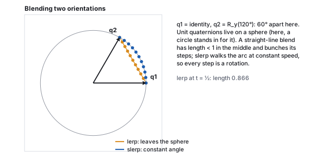
A unit circle with the identity q1 and the quaternion q2 of a 120 degree turn, 60 degrees apart on the circle; the straight-line lerp points in amber cut inside the circle, while the slerp points in blue sit evenly spaced along the arc.
Unit quaternions live on the unit sphere in four dimensions; a circle stands in for it. Every slerp step is a valid rotation and the steps are equal; the lerp steps are neither.
\[ \mathrm{slerp}(q_1, q_2, t) = \frac{\sin\big((1-t)\Omega\big)}{\sin\Omega}\,q_1 + \frac{\sin(t\,\Omega)}{\sin\Omega}\,q_2, \qquad \cos\Omega = q_1\cdot q_2 . \]

\(\Omega\) is the angle between the two quaternions in four dimensions, half the turn between the orientations (the half angle again).

(If \(q_1\cdot q_2 < 0\), negate one of them first: \(q\) and \(-q\) are the same rotation, and the short arc is the one between the nearer pair. For the pair below, using \(-q_2\) would give \(\cos\Omega = -0.5\), \(\Omega = 120^\circ\), and a swing of \(240^\circ\) the other way round.) Stepping an animation by composing the same small quaternion each frame is a discretized slerp; it is how a turntable, a door, or an orbiting camera is animated without ever touching a matrix, and the animation chapter measures slerp against the normalized-lerp shortcut, nlerp (normalize the straight blend): it walks the same arc at an uneven speed, \(27.8^\circ\) at \(t = 0.25\) where slerp has turned \(30^\circ\) for the pair below, with no sine or arccosine to evaluate.

See it live Blending orientations: scrub \(t\) under slerp, nlerp and the plain blend and compare the spacing of the dots; the inset is this section’s circle. Tick “use \(-q_2\)” and untick the sign check to see the long way round.
Worked example (slerp midpoint) From the identity \((0,0,0,1)\) to \(R_y(120^\circ)\), \(q_2 = (0, 0.866, 0, 0.5)\): \(\cos\Omega = 0.5\), \(\Omega = 60^\circ\), and at \(t = \tfrac12\) both weights are \(\sin 30^\circ / \sin 60^\circ = 0.577\), so the midpoint is \(0.577\,(0, 0.866, 0, 1.5) = (0, 0.5, 0, 0.866)\), which is exactly the quaternion of \(R_y(60^\circ)\): half the turn, as it should be. The plain average \((0, 0.433, 0, 0.75)\) has length \(0.866\) and is not a rotation.

6 · Euler angles and gimbal lock

The vocabulary comes from vehicles. Yaw turns about the up axis (look left or right), pitch about the side or wing axis (nose up or down), roll about the forward axis (bank). In Unity, with \(y\) up and \(z\) forward, yaw is about \(y\), pitch about \(x\) and roll about \(z\); aerospace puts \(x\) forward and \(z\) down, so there roll is about \(x\), pitch about \(y\) and yaw about \(z\). Same words, different letters.
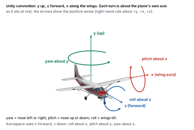
A Cessna 208 model with its three body axes: yaw about the up axis, pitch about the wing axis, roll about the forward axis, with curved arrows.
Yaw, pitch and roll in Unity’s convention (\(y\) up, \(z\) forward).

The human way to say an orientation: three rotations about three axes, in a fixed order. Unity’s Quaternion.Euler(x, y, z) applies \(Z\) first, then \(X\), then \(Y\), so the world-space product is \(R_y\,R_x\,R_z\). Three readable numbers, “pitch 20, yaw 45, roll 0”, but the order is a convention, and different tools pick different ones, which is the usual cause of an imported model arriving rotated wrong.
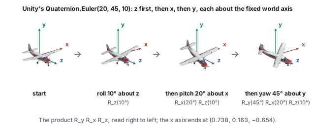
Four airplanes: at rest; rolled 10 degrees about z; then pitched 20 degrees about the world x; then yawed 45 degrees about the world y, which is Unity's Euler (20, 45, 10).
Unity’s Quaternion.Euler(20, 45, 10) as three turns about the fixed world axes, \(z\) first: the product \(R_y R_x R_z\) read right to left. The \(x\) axis ends at \((0.738, 0.163, -0.654)\), as in the worked example below. Computed with the library’s matrices.

6.1 Conventions

Twelve orders are possible (six with three distinct axes, six that repeat the first), each read either intrinsically (each rotation about the body’s own, already-rotated axis) or extrinsically (each about a fixed world axis). The two readings are the same product written in opposite order: intrinsic \(X\), then \(Y\), then \(Z\) is the matrix \(R_x R_y R_z\), which is also extrinsic \(Z\), then \(Y\), then \(X\). A library’s name for its order does not say which reading it means; the matrix does.

systemorder namematrix on a column vectorreads as
UnityZXY\(R_y\,R_x\,R_z\)\(Z\) first about the world axes, then \(X\), then \(Y\) (about the body: \(Y\), \(X\), \(Z\))
three.js default, and the library’s makeTRSXYZ\(R_x\,R_y\,R_z\)\(Z\) first about the world axes, then \(Y\), then \(X\) (about the body: \(X\), \(Y\), \(Z\))
aerospace (yaw, pitch, roll)ZYX\(R_z\,R_y\,R_x\)roll about world \(x\) first, then pitch, then yaw
Worked example (one triple, three matrices) The angles \((x, y, z) = (20^\circ, 45^\circ, 10^\circ)\) under the three conventions give three different orientations. Column 0 of each matrix, where the \(x\) axis lands: Unity’s \(R_y R_x R_z\) puts it at \((0.738, 0.163, -0.654)\); the library’s makeTRS(0,0,0, 20,45,10, 1,1,1), three.js order, at \((0.696, 0.401, -0.595)\); the aerospace order at \((0.696, 0.123, -0.707)\). The Unity and three.js orientations differ by a rotation of \(15.2^\circ\) (the angle of \(R_1^{\mathsf T}R_2\), by the log map of Appendix A.1), the Unity and aerospace ones by \(8.2^\circ\). Same three numbers, three poses.
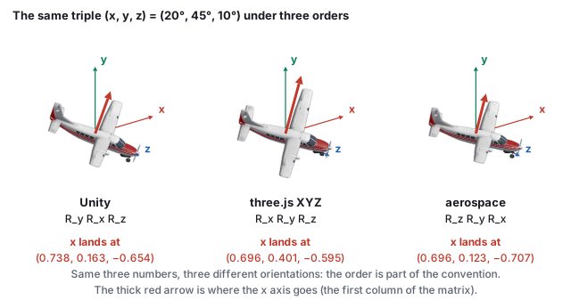
Three Cessna 208 models posed by the same angles (20, 45, 10) under Unity's, three.js's and the aerospace order, each labeled with where its x axis lands.
One triple, three conventions, three poses, computed with the library’s matrices: the \(x\) axis lands at \((0.738, 0.163, -0.654)\), \((0.696, 0.401, -0.595)\) and \((0.696, 0.123, -0.707)\).

6.2 Gimbals and the lock

A gimbal is a ring on two pins: it turns about one axis, the line through its pins. Nest three, each pinned inside the last, and the outer ring turns everything inside it while the inner one turns only the object. Three nested gimbals are a physical Euler-angle triple read intrinsically: the outer angle is the leftmost factor of the product, the inner angle the rightmost. The outer ring is pinned to the ground, so its axis is a world axis; the object is fixed to the inner ring, so that ring’s axis is one of the object’s own. Gyroscopes, camera heads and spacecraft inertial platforms are built this way, which is where the next failure got its name.
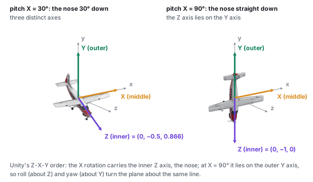
A Cessna 208 model and the three effective Euler axes for Unity's Z-X-Y order: at pitch 30 degrees the nose and the inner Z axis point to (0, -0.5, 0.866), distinct from the outer Y axis; at pitch 90 degrees the nose points straight down and the Z axis, (0, -1, 0), lies along the Y axis.
The effective axes of the three Euler rotations in the world, computed from the rotation matrices. The middle rotation (about \(X\)) carries the inner \(Z\) axis with it; at \(X = 90^\circ\) the inner axis has been tipped onto the outer one.
Worked example (where the inner axis goes) The inner rotation is about \(\hat{\mathbf{z}}\), but after the middle rotation \(R_x(x)\) its axis in the world is \(R_x(x)\,\hat{\mathbf{z}} = (0, -\sin x, \cos x)\). At \(x = 30^\circ\) that is \((0, -0.5, 0.866)\), a distinct direction. At \(x = 90^\circ\) it is \((0, -1, 0)\), the outer \(Y\) axis itself: the airplane’s nose axis now lies on the world’s \(y\) axis. Then rotating about \(Z\) and rotating about \(Y\) produce the same motion, three sliders give two effects, and one rotational degree of freedom is gone until \(x\) is backed off \(90^\circ\). That dead direction is gimbal lock.
See it live Euler angles on three gimbals: three nested rings carry a small airplane. Drag the pitch to \(90^\circ\) and press “wiggle outer” and “wiggle inner”: both turn the airplane about the same world axis. Back the pitch off to \(30^\circ\) and the two wiggles differ. Then set \((89^\circ, 0, 0)\) and press “fin y”, which turns the airplane itself \(1^\circ\) about its own up axis and reads the angles back: the airplane barely moves while the outer and inner rings swing \(45^\circ\) each (Section 6.3). Switch the order to three.js and the lock moves to the middle angle of that order, \(y\).

6.3 What locks: the angles, not the airplane

The two axes that line up at the lock are not two of the airplane’s axes. Those stay perpendicular at every pose, and turning the airplane about any of them always works: a program that keeps the orientation as a quaternion or a matrix and multiplies in a small turn about the body’s own axis, \(R \leftarrow R\,R_{\text{axis}}(\delta)\), can turn any way from any pose and never locks. That is how engines and physics apply rotation (Unity’s transform.rotation * Quaternion.AngleAxis(d, Vector3.up), three.js’s object.rotateY(d)). The axes that line up are the outer ring’s, fixed in the world, and the inner ring’s, fixed in the airplane.

What fails is the description by three angles. A program whose state is the triple \((x, y, z)\) (an inspector, an animation curve on Euler channels, a camera kept as yaw and pitch) has to express every turn as changes of the three numbers, and near the lock some turns need enormous changes.

Worked example (how fast the angles must move) To first order two small turns compose by adding their rotation vectors \(\theta\hat{\mathbf{n}}\) (multiply \(I + aK_1\) by \(I + bK_2\) and drop the product term; Appendix A.2). So a small change \((dx, dy, dz)\) of Unity’s angles turns the object by \(dy\,\hat{\mathbf{y}} + dx\,\hat{\mathbf{x}} + dz\,(0, -\sin x, \cos x)\), each change about its gimbal’s axis in the world (take \(y = 0\); a nonzero \(y\) turns the whole picture about \(\hat{\mathbf{y}}\) and changes none of the numbers). Now turn the airplane by a small angle \(d\theta\) about its own fin axis, which in the world is \(R_x(x)\,\hat{\mathbf{y}} = (0, \cos x, \sin x)\). Matching components: \(dx = 0\), \(dz\cos x = d\theta\sin x\) and \(dy - dz\sin x = d\theta\cos x\), so \[ dz = \tan x \; d\theta, \qquad dy = \frac{d\theta}{\cos x}. \] At \(x = 20^\circ\) that is \(dy = 1.06\,d\theta\) and \(dz = 0.36\,d\theta\); at \(80^\circ\), \(5.76\,d\theta\) and \(5.67\,d\theta\); at \(90^\circ\) no change of the angles does it, which is the dead direction of the previous example. For a whole \(1^\circ\) turn, read back with the extraction of Appendix A.4: at \(x = 89^\circ\) the angles move \(y\) by \(45^\circ\) and \(z\) by \(45^\circ\); at \(x = 90^\circ\) they move \(90^\circ\) each, however small the turn. Code: eulerFromMatrix('unity', matMul(eulerMatrix('unity', 89, 0, 0), axisRot('y', 1))) (lib/core/rot-reps.js, with matMul from lib/core/xform.js) returns \((88.59, 45.00, 45.00)\).

A physical gimbal is that program in hardware: its three ring angles are the state. To hold an inertial platform still while the spacecraft turns about the dead direction, the gimbal motors would have to turn \(1/\cos x\) times as fast as the craft, so the Apollo crews flew around the lock orientation. Nothing is wrong with the orientation at pitch \(90^\circ\); the object is fine. It is the chart \((\text{yaw}, \text{pitch}, \text{roll})\) that goes singular there (a chart is a set of coordinates laid over the rotations, as latitude and longitude are laid over the globe), the way longitude is undefined at the poles: one step at the North Pole can change your longitude by \(90^\circ\). A quaternion names an axis and an angle with no nested frames, so there is no configuration where two of its parts align. That is the engineering reason engines store the quaternion and show Euler angles only for editing: transform.rotation is a quaternion under the hood, always. Cameras that do keep yaw and pitch as their state clamp the pitch short of \(\pm 90^\circ\).

7 · Choosing a representation

matrix \(3\times3\)axis-anglequaternionEuler angles
numbers stored94 (or 3, as \(\theta\hat{\mathbf{n}}\))43
constraints61 (unit axis)1 (unit length)0
apply to a point9 multipliesvia Rodrigues, about 20via the sandwich, about 20; or convert onceconvert first
compose27 multipliesconvert first16 multipliesconvert first
inverttransposenegate \(\theta\)conjugatenegate and reverse the order
interpolatenoawkwardslerpbadly (Section 6, and the animation chapter)
singularitiesnoneaxis undefined at \(\theta = 0\)none (a double cover)gimbal lock
drift under compositionshearsnone storedlength only, one divide fixes itnone stored
readable by a personcolumns are axesyesnoyes

The practice that follows from the table: store and interpolate a quaternion, compose quaternions, convert to a matrix once per frame for the GPU, show Euler angles in the inspector, and use axis-angle when the physics hands you an angular velocity. Every conversion in that pipeline is in this chapter. The fifth name, “turn this direction onto that one” (Section 5.1), is a way to build a rotation rather than to store one; it produces a quaternion.

See it live One rotation, five definitions: define the rotation by its columns, an axis and angle, a quaternion, Euler angles or a from-to pair, and read the other four live. Every mode starts at \(R_y(30^\circ)\), so switching modes changes the controls and not the cube.

8 · In code

Hands-on Run these from the css551/ directory. The library stores matrices column-major as 16-element arrays (the affine chapter explains the layout), so the first four printed numbers are column 0.
  1. The matrix and quaternion of the chapter’s rotation:
    node -e "import('./lib/core/xform.js').then(x=>{const R=x.axisAngleMatrix(0,1,0,30);console.log(R.map(v=>+v.toFixed(3)));console.log(x.quatFromAxisAngle(0,1,0,30).map(v=>+v.toFixed(3)));})"
    [ 0.866, 0, -0.5, 0,  0, 1, 0, 0,  0.5, 0, 0.866, 0,  0, 0, 0, 1 ]
    [ 0, 0.259, 0, 0.966 ]
  2. Orthonormal columns: column 0 dotted with itself and with column 2 (Section 1.1):
    node -e "import('./lib/core/xform.js').then(x=>{const R=x.axisAngleMatrix(0,1,0,30);const c0=[R[0],R[1],R[2]],c2=[R[8],R[9],R[10]];console.log(x.dot(c0,c0).toFixed(6), x.dot(c0,c2).toFixed(6));})"
    1.000000 0.000000
  3. The diagonal axis permutes the basis and fixes the cube’s corner (Section 3.1):
    node -e "import('./lib/core/xform.js').then(x=>{const R=x.axisAngleMatrix(1,1,1,120);console.log(x.applyMat4(R,[1,0,0]).slice(0,3).map(v=>+v.toFixed(3)), x.applyMat4(R,[1,1,1]).slice(0,3).map(v=>+v.toFixed(3)));})"
    [ 0, 1, -0 ] [ 1, 1, 1 ]
  4. The angle of the composite \(R_x(30^\circ)R_y(30^\circ)\) from its trace (Appendix A.1):
    node -e "import('./lib/core/xform.js').then(x=>{const M=x.matMul(x.axisAngleMatrix(1,0,0,30),x.axisAngleMatrix(0,1,0,30));const tr=M[0]+M[5]+M[10];console.log((Math.acos((tr-1)/2)*180/Math.PI).toFixed(2));})"
    42.18
  5. Extract Unity-order Euler angles from a matrix built in that order (Appendix A.4); then change the 20 to 90 and watch \(y\) and \(z\) come back as noise:
    node -e "import('./lib/core/xform.js').then(x=>{const e=(a,b,c)=>x.matMul(x.matMul(x.axisAngleMatrix(0,1,0,b),x.axisAngleMatrix(1,0,0,a)),x.axisAngleMatrix(0,0,1,c));const M=e(20,45,10);const m=(r,c)=>M[4*c+r];console.log((Math.asin(-m(1,2))*180/Math.PI).toFixed(2),(Math.atan2(m(0,2),m(2,2))*180/Math.PI).toFixed(2),(Math.atan2(m(1,0),m(1,1))*180/Math.PI).toFixed(2));})"
    20.00 45.00 10.00
  6. In the axis-angle demo, set the angle to \(180^\circ\) and read \(w\) in the quaternion panel: it is 0, and the axis components carry everything. Then set \(360^\circ\): the quaternion is \((0, 0, 0, -1)\), the double cover of the identity.

9 · Exercises

Exercise 1 (columns) Write \(R_z(90^\circ)\) by reading where the axes land, without the formula.
Solution A right-handed quarter turn about \(z\) sends \(\hat{\mathbf{x}}\) to \(\hat{\mathbf{y}}\), \(\hat{\mathbf{y}}\) to \(-\hat{\mathbf{x}}\), and leaves \(\hat{\mathbf{z}}\). Columns \((0,1,0)\), \((-1,0,0)\), \((0,0,1)\), so \(R_z(90^\circ) = \begin{pmatrix} 0 & -1 & 0 \\ 1 & 0 & 0 \\ 0 & 0 & 1 \end{pmatrix}\).
Exercise 2 (Rodrigues) Rotate \(\mathbf{v} = (1, 1, 0)\) by \(90^\circ\) about \(\hat{\mathbf{n}} = (0, 0, 1)\) with Rodrigues’ formula, and check with the column reading.
Solution \(\mathbf{v}\cdot\hat{\mathbf{n}} = 0\), \(\hat{\mathbf{n}}\times\mathbf{v} = (0\cdot0 - 1\cdot1,\; 1\cdot1 - 0\cdot0,\; 0) = (-1, 1, 0)\); \(\cos 90^\circ = 0\), \(\sin 90^\circ = 1\), so \(\mathbf{v}' = (-1, 1, 0)\). By columns: \(\hat{\mathbf{x}}\to\hat{\mathbf{y}}\) and \(\hat{\mathbf{y}}\to-\hat{\mathbf{x}}\), so \((1,1,0)\to(0,1,0) + (-1,0,0) = (-1, 1, 0)\).
Exercise 3 (quaternion) Write the quaternion for \(180^\circ\) about \((1, 1, 0)/\sqrt2\), and use the sandwich formula to rotate \((1, 0, 0)\).
Solution Half angle \(90^\circ\): \(q = (0.707, 0.707, 0, 0)\), \(w = 0\). \(\mathbf{q}_v\times\mathbf{p} = (0.707, 0.707, 0)\times(1,0,0) = (0, 0, -0.707)\); the \(2w\) term vanishes; \(\mathbf{q}_v\times(0, 0, -0.707) = (0.707\cdot(-0.707) - 0,\; 0 - 0.707\cdot(-0.707),\; 0) = (-0.5, 0.5, 0)\); doubled, \((-1, 1, 0)\); sum \((0, 1, 0)\). A half turn about the diagonal swaps \(x\) and \(y\).
Exercise 4 (composition) Show that \(q_y\,q_x \ne q_x\,q_y\) for the two \(30^\circ\) quaternions of Section 5 by computing the \(z\) component of each.
Solution With \(q_x = (a, 0, 0, c)\) and \(q_y = (0, a, 0, c)\), \(a = 0.259\), \(c = 0.966\): \((q_x q_y)_z = x_1 y_2 - y_1 x_2 = a\cdot a - 0 = 0.067\) and \((q_y q_x)_z = 0 - a\cdot a = -0.067\). Opposite signs: the two orders differ, as they must.
Exercise 5 (the lock, in another order) For an \(X\)-\(Y\)-\(Z\) order (world product \(R_z R_y R_x\)), which angle locks, and at what value?
Solution The middle angle, \(Y\), at \(\pm90^\circ\): the inner \(X\) axis becomes \(R_y(90^\circ)\hat{\mathbf{x}} = (0, 0, -1)\), parallel to the outer \(Z\) axis. In every order it is the middle rotation at a quarter turn that aligns the inner and outer axes.
Exercise 6 (properties) The matrix with columns \((0.6, 0.8, 0)\), \((-0.8, 0.6, 0)\), \((0, 0, -1)\) has orthonormal columns. Is it a rotation? If not, write it as a rotation times a mirror.
Solution The determinant is \(0.6\cdot0.6\cdot(-1) - (-0.8)\cdot0.8\cdot(-1) = -0.36 - 0.64 = -1\): a reflection. It is \(R_z(53.13^\circ)\) (the first two columns, \(\cos\theta = 0.6\)) followed by the mirror \(\mathrm{diag}(1, 1, -1)\), which flips \(z\). A mesh transformed by it turns inside out.
Exercise 7 (the half angle and the double cover) Write the quaternion for \(R_y(360^\circ)\) and for \(R_y(720^\circ)\). Which matrix does each give, and what does the first one say about the half angle?
Solution Half angles \(180^\circ\) and \(360^\circ\): \(q = (0, \sin 180^\circ, 0, \cos 180^\circ) = (0, 0, 0, -1)\) and \((0, 0, 0, 1)\). Both give the identity matrix (the sandwich \(q\,p\,q^{-1}\) uses \(q\) twice, so the sign cancels). A full turn of the object is half a lap of \(q\): \(q\) has reached minus the identity and needs a second full turn to come home. Check it in the axis-angle demo’s half-angle layer.
Exercise 8 (from one direction to another, with code) Find the quaternion that turns \((0, 0, 1)\) onto \((1, 0, 0)\) with the formula of Section 5.1, by hand, then check it with fromTo in lib/core/rot-reps.js.
Solution \(\mathbf{a}\cdot\mathbf{b} = 0\), \(\mathbf{a}\times\mathbf{b} = (0\cdot0 - 1\cdot0,\; 1\cdot1 - 0\cdot0,\; 0\cdot0 - 0\cdot1) = (0, 1, 0)\), so \(q = \mathrm{normalize}(0, 1, 0, 1) = (0, 0.707, 0, 0.707)\): \(90^\circ\) about \(y\), and indeed \(R_y(90^\circ)\) has column 2 equal to \((1, 0, 0)\). Code: node -e "import('./lib/core/rot-reps.js').then(r=>console.log(r.fromTo([0,0,1],[1,0,0]).q.map(v=>+v.toFixed(3))))" prints [ 0, 0.707, 0, 0.707 ].

Appendix

A.1 The log map: axis and angle from a matrix

The trace of a matrix is the sum of its diagonal entries. For a rotation it has a picture. Diagonal entry \(i\) is \(\mathbf{e}_i\cdot(R\mathbf{e}_i)\): how much of axis \(i\) is still pointing along itself after the turn. Measure with a frame lined up with the rotation, one axis along \(\hat{\mathbf{n}}\) and two in the plane across it: the axis keeps all of itself (1), and each in-plane direction keeps \(\cos\theta\) of itself. The trace is the same in every orthonormal frame (a change of frame is \(R\mapsto Q^{\mathsf T}RQ\), and the trace of a product does not change when its factors are cycled), so \(\mathrm{tr}\,R = 1 + 2\cos\theta\) whatever the axis. For \(R_y(30^\circ)\): \(0.866 + 1 + 0.866 = 2.732 = 1 + 2(0.866)\).
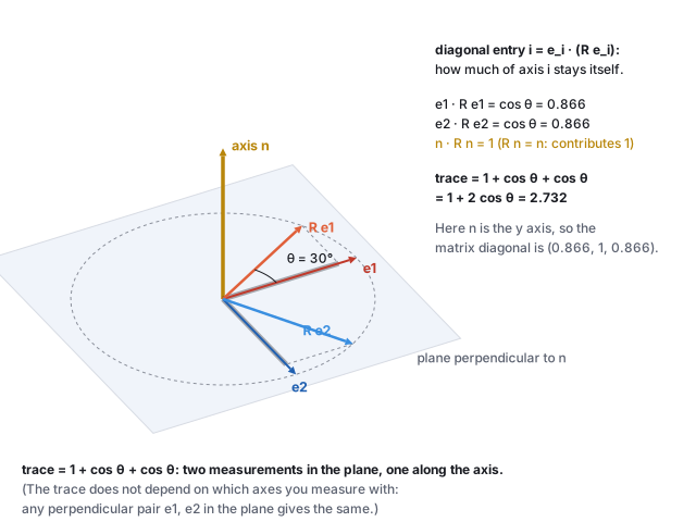
The rotation axis n unchanged, and two perpendicular unit vectors e1 and e2 in the plane across it with their images R e1 and R e2 turned by theta; the projection of each image back onto the original is cos theta.
Why \(\mathrm{tr}\,R = 1 + 2\cos\theta\): the axis keeps all of itself, each of two perpendicular in-plane directions keeps \(\cos\theta\) of itself. Computed from the library’s matrix for the drawn angle.

The same fact, from the matrix form: the trace of \(R\) is \(3 + 0 + (1 - \cos\theta)\,\mathrm{tr}(K^2)\), and \(\mathrm{tr}(K^2) = -2\) for a unit axis, so \(\mathrm{tr}\,R = 1 + 2\cos\theta\). The symmetric part of \(R\) is \(I + (1 - \cos\theta)K^2\) and the antisymmetric part (half of \(R - R^{\mathsf T}\), the matrix minus its transpose, which keeps only the off-diagonal differences) is \(\sin\theta\,K\), from which the axis can be read entry by entry:

Axis and angle from a rotation matrix \[ \cos\theta = \frac{\mathrm{tr}\,R - 1}{2}, \qquad \hat{\mathbf{n}} = \frac{1}{2\sin\theta}\,\big(R_{21} - R_{12},\; R_{02} - R_{20},\; R_{10} - R_{01}\big) . \] The second formula divides by \(\sin\theta\) and fails as \(\theta\to180^\circ\); there the axis is recovered from the symmetric part instead, \(n_i^2 = (R_{ii} + 1)/2\).
Worked example (the product of Section 5, read as one rotation) \(R = R_x(30^\circ)\,R_y(30^\circ)\) has rows \((0.866, 0, 0.5)\), \((0.25, 0.866, -0.433)\), \((-0.433, 0.5, 0.75)\). Trace \(2.482\), so \(\cos\theta = 0.741\), \(\theta = 42.18^\circ\). The antisymmetric differences are \((0.5 - (-0.433),\; 0.5 - (-0.433),\; 0.25 - 0) = (0.933, 0.933, 0.25)\), and dividing by \(2\sin\theta = 1.343\) gives \(\hat{\mathbf{n}} = (0.695, 0.695, 0.186)\), a unit vector. The quaternion route in Section 5 finds the same \(42.18^\circ\) about the same axis. Two ways in, one rotation out.
Pitfall Reading the axis from \(R - R^{\mathsf T}\) near a half turn. For \(R_y(\theta)\) the antisymmetric vector has length \(2\sin\theta\): \(0.347\) at \(170^\circ\), \(0.035\) at \(179^\circ\), \(0.0035\) at \(179.9^\circ\), and \(2\times10^{-16}\) (round-off) at exactly \(180^\circ\). Dividing a vector of round-off noise by another round-off number gives an axis pointing anywhere. The symmetric part is unaffected: at \(180^\circ\), \(\sqrt{(R_{ii} + 1)/2}\) gives \((0, 1, 0)\), the true axis up to sign. A conversion routine must branch on the angle; the quaternion extraction of Appendix A.3 branches for the same reason.

A.2 Small angles, and the angular velocity

For small \(\theta\) (in radians), \(\sin\theta\approx\theta\) and \(1 - \cos\theta\approx\theta^2/2\), so \(R \approx I + \theta K + \tfrac12\theta^2K^2\), and to first order (keeping the terms proportional to \(\theta\) and dropping \(\theta^2, \theta^3, \ldots\)) \(R\mathbf{v}\approx\mathbf{v} + \theta\,\hat{\mathbf{n}}\times\mathbf{v}\): a small turn moves every point along the tangent \(\hat{\mathbf{n}}\times\mathbf{v}\) of its circle. That is the physics of spinning: a body turning about \(\hat{\mathbf{n}}\) at rate \(\omega\) has angular velocity \(\boldsymbol\omega = \omega\hat{\mathbf{n}}\), and a point at \(\mathbf{p}\) on it moves with velocity \(\boldsymbol\omega\times\mathbf{p}\). The exact rotation is the limit of many small ones, \(R = \exp(\theta K)\), the matrix exponential, defined by the same power series as \(e^x\): \(\exp(A) = I + A + A^2/2! + A^3/3! + \cdots\). For \(A = \theta K\), \(K^3 = -K\) folds every power back onto \(K\) or \(K^2\), the odd terms sum to \(\sin\theta\,K\) and the even ones to \((1 - \cos\theta)K^2\), which is Rodrigues again. That is why the axis-angle vector \(\theta\hat{\mathbf{n}}\) is called the exponential coordinate of a rotation and Appendix A.1 its logarithm.
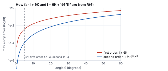
A log plot of the largest entry error against the angle from 0 to 60 degrees for two approximations of R_y(theta): the first-order I plus theta K, and the second-order one adding half theta squared K squared; the second is about a hundred times better at 5 degrees.
How wrong the truncated series is. At \(5^\circ\) the first-order matrix is off by \(3.8\times10^{-3}\) in its worst entry, the second-order by \(1.1\times10^{-4}\); at \(30^\circ\) by \(0.13\) and \(0.024\). The first-order matrix is not a rotation at all: its columns have length \(1.004\) at \(5^\circ\) and \(1.13\) at \(30^\circ\).
Worked example (one physics step) A wheel spins at \(90^\circ\) per second about \(y\): \(\boldsymbol\omega = (0, 1.571, 0)\) rad/s. The point \(\mathbf{p} = (1, 0, 0)\) on its rim has velocity \(\boldsymbol\omega\times\mathbf{p} = (0, 0, -1.571)\), speed \(1.571\) (radius times rate). One frame of \(1/60\) s by the first-order step, \(\mathbf{p} + \Delta t\,\boldsymbol\omega\times\mathbf{p} = (1, 0, -0.0262)\), has length \(1.00034\): the point has drifted off the rim by \(3.4\times10^{-4}\). The exact step \(R_y(1.5^\circ)\,\mathbf{p} = (0.9997, 0, -0.0262)\) keeps it on. Sixty such steps a second is the drift measured in Appendix A.5, and the animation chapter shows the same effect in a spring.
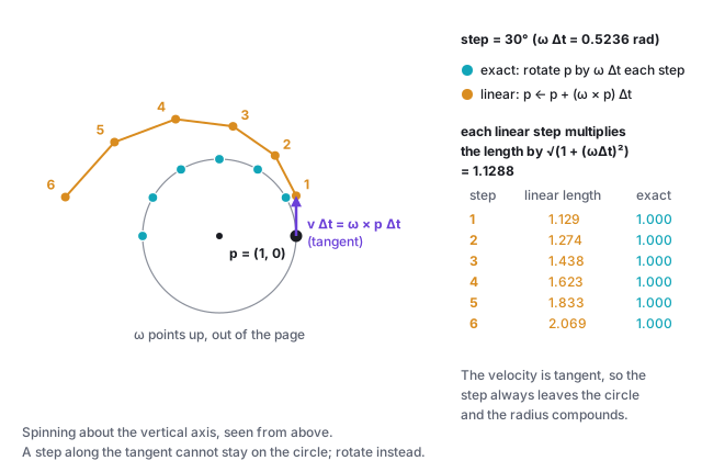
Top view of a unit circle: a point p, its tangent velocity, a linear step landing outside the circle, and repeated linear steps spiralling outward while exact steps stay on the circle.
The linear step, drawn with a large step so it shows: each step is along the tangent, perpendicular to \(\mathbf{p}\), so by Pythagoras it multiplies the length by \(\sqrt{1 + (\omega\Delta t)^2}\). Exact steps stay on the circle.
Pitfall Stepping a spin with the linear rule. The update \(\mathbf{p}\leftarrow\mathbf{p} + \Delta t\,(\boldsymbol\omega\times\mathbf{p})\), where \(\Delta t\) is the time one frame advances (an explicit Euler step: move along the current velocity for one time step), multiplies the length by \(\sqrt{1 + (\omega\Delta t)^2}\) every frame, and the error compounds: at \(90^\circ\) per second and 60 steps per second the point is at radius \(1.000343\) after one step, \(1.0208\) after one second, and \(1.2282\) after ten. A spinning object integrated this way spirals outward. Step the orientation instead, by the rotation of \(\boldsymbol\omega\Delta t\) (as a quaternion, Section 4), and renormalize.
See it live Angular velocity: stepping a spin: two points start at \((1, 0, 0)\) on a turntable; one takes the linear step, one the exact rotation per frame. Scrub the time to 1 s and 10 s and read the two radii; lower the steps per second to 4 to see the spiral at a glance.

A.3 Quaternion to matrix, and matrix to quaternion

Apply the sandwich to the three basis vectors and the columns of the matrix come out as polynomials in the four components. That is how an engine turns the stored quaternion into the matrix the GPU needs, every frame, with no trigonometry:

Quaternion to matrix \[ R(q) = \begin{pmatrix} 1 - 2(y^2 + z^2) & 2(xy - zw) & 2(xz + yw) \\ 2(xy + zw) & 1 - 2(x^2 + z^2) & 2(yz - xw) \\ 2(xz - yw) & 2(yz + xw) & 1 - 2(x^2 + y^2) \end{pmatrix}. \] Going back, the trace is \(3 - 4(x^2 + y^2 + z^2) = 4w^2 - 1\), so \(w = \tfrac12\sqrt{1 + \mathrm{tr}\,R}\), and the off-diagonal differences give \(x = (R_{21} - R_{12})/4w\) and its cyclic siblings. When \(w\) is small the division loses digits, so a robust routine (Shepperd’s method, 1978) picks whichever of \(w, x, y, z\) is largest from the diagonal, computes that one by a square root, and divides the others by it.
Worked example (both directions) Forward, from \(q = (0, 0.259, 0, 0.966)\): the entry \((0, 0)\) is \(1 - 2(0.259^2 + 0) = 1 - 0.134 = 0.866\) and the entry \((0, 2)\) is \(2(0 + 0.259\cdot0.966) = 0.5\); all nine give the \(R_y(30^\circ)\) of Section 2, with no cosine evaluated. Backward, on the product matrix of Appendix A.1 (trace \(2.482\)): \(w\) is the largest candidate, \(s = 2\sqrt{1 + 2.482} = 3.732\), \(w = s/4 = 0.933\), \(x = (R_{21} - R_{12})/s = 0.933/3.732 = 0.25\), \(y = 0.25\), \(z = 0.25/3.732 = 0.067\): \(q = (0.25, 0.25, 0.067, 0.933)\), the quaternion product Section 5 computes directly. For \(R_y(180^\circ)\) the trace is \(-1\), \(w = 0\), and the routine branches to the \(y\) diagonal entry to get \((0, 1, 0, 0)\).

A.4 Extracting Euler angles from a matrix

Multiplying out \(R_y(y)\,R_x(x)\,R_z(z)\) puts single trigonometric factors in three places: the entry \((1, 2)\) is \(-\sin x\), the entries \((0, 2)\) and \((2, 2)\) are \(\sin y\cos x\) and \(\cos y\cos x\), and the entries \((1, 0)\) and \((1, 1)\) are \(\cos x\sin z\) and \(\cos x\cos z\). So, with \(\mathrm{atan2}(s, c)\) the angle whose sine and cosine are in the ratio \(s : c\), in all four quadrants,

\[ x = \arcsin(-R_{12}), \qquad y = \mathrm{atan2}(R_{02}, R_{22}), \qquad z = \mathrm{atan2}(R_{10}, R_{11}), \]

and the extraction is exact as long as \(\cos x \ne 0\).

Worked example (extraction, and the lock) For \((20^\circ, 45^\circ, 10^\circ)\) the matrix has \(R_{12} = -0.342\), \(R_{02} = R_{22} = 0.6645\), \(R_{10} = 0.163\), \(R_{11} = 0.925\): \(x = \arcsin 0.342 = 20^\circ\), \(y = \mathrm{atan2}(0.6645, 0.6645) = 45^\circ\), \(z = \mathrm{atan2}(0.163, 0.925) = 10^\circ\). Now \((90^\circ, 45^\circ, 10^\circ)\): \(R_{12} = -1\) gives \(x = 90^\circ\), but \(R_{02}, R_{22}, R_{10}, R_{11}\) are all zero, and \(\mathrm{atan2}(0, 0)\) is meaningless. What survives is the difference \(y - z\): the matrix’s first row is \((\cos(y - z), \sin(y - z), 0)\), and \(\mathrm{atan2}(R_{01}, R_{00}) = 35^\circ\). The triple \((90^\circ, 25^\circ, 30^\circ)\) has first row \((0.996, -0.087, 0)\) and \(y - z = -5^\circ\): a different orientation, but at the lock only the difference \(y - z\) is observable, and \((90^\circ, 60^\circ, 25^\circ)\) would be the same orientation as the first triple. A converter must choose one triple for it (Unity sets \(z = 0\) and puts everything in \(y\)), which is why an inspector shows a pitched-up object with angles that jump.

Even away from the lock, a matrix has two Euler triples: \((20^\circ, 45^\circ, 10^\circ)\) and \((160^\circ, 225^\circ, 190^\circ)\) produce the same matrix, since \(x\mapsto180^\circ - x\) with \(180^\circ\) added to the other two is the same orientation. The extraction above always returns the one with \(x\in[-90^\circ, 90^\circ]\).

A.5 Drift, measured

The claim “matrices drift” can be measured. Compose the same \(1^\circ\) rotation 200,000 times in single-precision arithmetic three ways: as a \(3\times3\) matrix product, as a quaternion product, and as a quaternion product renormalized after every step.
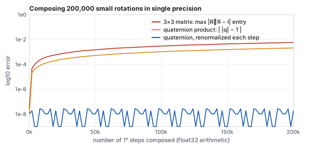
A log-scale plot of error against the number of 1-degree steps composed in float32: the matrix orthogonality error grows to about 6e-3 by 200,000 steps, the raw quaternion length error to about 2e-3, and the renormalized quaternion stays at the 1e-8 floor of single precision.
Single-precision arithmetic (every operation rounded to float32), 200,000 compositions of \(R_y(1^\circ)\). The matrix’s columns stop being orthonormal by \(6\times10^{-3}\), enough to shear a model visibly; the quaternion’s length drifts by \(2\times10^{-3}\), and one division per step removes it entirely.

The matrix needs six constraints re-imposed (a full re-orthonormalization, which is the Gram–Schmidt of the vectors chapter applied to its columns); the quaternion needs one (divide by its length), and that is cheap enough to do every frame. A game running at 60 frames per second accumulates 200,000 compositions in under an hour.

Pitfall Accumulating instead of recomputing. The drift above comes from applying a delta to the stored state, \(R \leftarrow R\,\Delta R\), thousands of times. The alternative that never drifts is to keep the parameters (an angle, or a quaternion that is renormalized) and rebuild the matrix from them each frame; a turntable stored as an angle \(\theta\) that grows by \(1^\circ\) a frame and is turned into \(R_y(\theta)\) fresh is exact forever, since \(\theta\) is a single float with no constraint to lose. Every demo on the course site works this way, and it is the model–view discipline of the interaction chapter: the matrix is a view of the model, never the model.

A.6 Exercises

Exercise A1 (the log map) The matrix \(\begin{pmatrix} 0 & 0 & 1 \\ 1 & 0 & 0 \\ 0 & 1 & 0 \end{pmatrix}\) of Section 3.1: recover its angle and axis from the trace and the antisymmetric part.
Solution Trace 0, so \(\cos\theta = -\tfrac12\), \(\theta = 120^\circ\), \(2\sin\theta = 1.732\). Differences \((R_{21} - R_{12}, R_{02} - R_{20}, R_{10} - R_{01}) = (1 - 0, 1 - 0, 1 - 0) = (1, 1, 1)\), divided by \(1.732\): \((0.577, 0.577, 0.577)\), the diagonal. The formula returns exactly the axis and angle the matrix was built from.
Exercise A2 (conversion) Convert \(q = (0.5, 0.5, 0.5, 0.5)\) to a matrix. What rotation is it?
Solution Unit length: \(4\times0.25 = 1\). Entry \((0,0)\): \(1 - 2(0.25 + 0.25) = 0\); entry \((1,0)\): \(2(xy + zw) = 2(0.25 + 0.25) = 1\); entry \((2,0)\): \(2(xz - yw) = 0\). Column 0 is \((0, 1, 0)\), and the other columns follow the same way: the permutation matrix of Section 3.1. Indeed \(w = \cos\tfrac\theta2 = 0.5\) gives \(\theta = 120^\circ\), and the vector part \((0.5, 0.5, 0.5) = \sin 60^\circ\cdot(1,1,1)/\sqrt3\) is the diagonal axis.
Exercise A3 (small angles, with code) For \(\theta = 2^\circ\), compute the first-order matrix \(I + \theta K\) for the \(y\) axis by hand and its column-0 length. Then check the exact matrix with axisAngleMatrix(0,1,0,2) and report the largest entry difference.
Solution \(\theta = 0.0349\) rad; \(K\) for \(\hat{\mathbf{y}}\) has \(K_{02} = 1\), \(K_{20} = -1\), so \(I + \theta K\) has rows \((1, 0, 0.0349)\), \((0,1,0)\), \((-0.0349, 0, 1)\); column 0 has length \(\sqrt{1 + 0.0349^2} = 1.00061\). The exact matrix has \(\cos 2^\circ = 0.99939\) on the diagonal, so the largest difference is \(6.1\times10^{-4}\), in line with the figure of Appendix A.2 (\(1.5\times10^{-4}\) at \(1^\circ\), growing as \(\theta^2\)). Code: node -e "import('./lib/core/xform.js').then(x=>{const R=x.axisAngleMatrix(0,1,0,2);console.log((1-R[0]).toExponential(2));})" prints 6.09e-4.
Exercise A4 (Euler extraction, with the demo or code) Build the Unity-order matrix for \((x, y, z) = (-30^\circ, 120^\circ, 200^\circ)\) with the hands-on snippet and extract the angles. Why is the result not the input, and is it the same orientation?
Solution The extraction returns \((-30^\circ, 120^\circ, -160^\circ)\): \(\mathrm{atan2}\) reports angles in \((-180^\circ, 180^\circ]\), and \(200^\circ\) and \(-160^\circ\) are the same rotation about \(z\). Had \(x\) been outside \([-90^\circ, 90^\circ]\), the routine would have returned the other triple of Appendix A.4 instead. Both are the same orientation; the numbers are a chart, not the thing.
Exercise A5 (the linear step, with the demo) A point at radius 1 spins at \(180^\circ\) per second and is stepped with \(\mathbf{p}\leftarrow\mathbf{p} + \Delta t\,(\boldsymbol\omega\times\mathbf{p})\) at 30 steps per second. What is its radius after one second? Check it in the spin-step demo.
Solution \(\omega\Delta t = \pi/30 = 0.1047\) rad per step; each step multiplies the length by \(\sqrt{1 + 0.1047^2} = 1.00547\), and 30 steps give \(1.00547^{30} = 1.178\): 18 percent too far out after one half turn. Halving the step (60 per second) gives \(\sqrt{1 + 0.0524^2}^{\,60} = 1.086\): the error shrinks with the step but never vanishes. The quaternion step stays at radius 1.