This chapter links to the course’s interactive demos and to original papers on the open web, and it uses MathJax for its formulas. Read it through the course website (or download the file and open it in a browser); a Canvas inline preview will reach neither the demos nor the math. All chapters.
Inverse and Differentiable Rendering
“All models are wrong, but some are useful.” George Box, Robustness in the Strategy of Scientific Model Building, 1979
A renderer maps a scene’s parameters (shapes, materials, lights, camera) to an image. Inverse rendering asks for the parameters given the image. The modern answer is to make the renderer differentiable and descend the gradient of an image loss: render, compare with the photograph, push the error back through every pixel to every parameter, and repeat. Shading and lighting differentiate by the chain rule. Visibility does not: a pixel is inside an object or outside it, and the derivative of that step is zero almost everywhere, so a naive differentiable renderer cannot see an edge move. The four families of fixes (edge sampling, reparameterization, path-space boundary integrals, and soft rasterization) are the core of the field, and the systems built on them (Mitsuba 3 and Dr.Jit) recover materials, lights, geometry and volumes from photographs. Every worked number below comes from the course’s own 64 × 64 differentiable renderer, the engine of the inverse-render demo.
- Rendering as a function
- The inverse problem, and why it is ill-posed
- Analysis by synthesis
- Automatic differentiation: forward and reverse
- Differentiating shading and lighting
- The visibility discontinuity
- Four answers to the edge problem
- Differentiable path tracers
- What can be recovered
- NeRF and splatting as inverse rendering
- Regularization and priors
- Open problems
- The papers
- Exercises
1 · Rendering as a function
Every renderer in this text, the rasterizer of the rasterization chapter and the path tracer of the ray-tracing chapter alike, computes a function from numbers that describe a scene to numbers that describe an image.
The course renderer has \(m = 8\): an RGB albedo \(\rho\), a light direction given by azimuth and elevation, \(\mathbf{l} = (\cos\phi_e \sin\phi_a,\ \sin\phi_e,\ \cos\phi_e\cos\phi_a)\), and a sphere’s radius \(r\) and center \((c_x, c_y)\), seen by an orthographic camera on a \(64 \times 64\) grid over \([-1,1]^2\). A pixel center at distance \(d\) from the center is covered when \(d < r\); there the normal is \(\mathbf{n} = (d_x, d_y, \sqrt{r^2 - d^2})/r\), and the color is \[ P = a\,S + (1-a)\,B, \qquad S = \rho\,\big(k_a + E\max(0, \mathbf{n}\cdot\mathbf{l})\big), \] with coverage \(a \in \{0, 1\}\), background \(B = (0.10, 0.12, 0.16)\), ambient \(k_a = 0.08\) and light intensity \(E = 1\): the Lambert model of the illumination chapter on the ray–sphere geometry of the ray-tracing chapter. The output has \(3 \cdot 64^2 = 12{,}288\) numbers.
2 · The inverse problem, and why it is ill-posed
Hadamard called a problem well-posed when a solution exists, is unique, and depends continuously on the data. Inverse rendering fails the second test routinely and the third often.
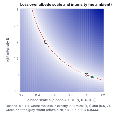
The albedo–intensity product is the simplest of many such families. Shape and shading trade off (a darker patch is either darker paint or a surface turned away from the light); the bas-relief ambiguity lets a flattened shape under a moved light produce the same shaded image; a mirror reflects an environment that cannot be told apart from a texture painted on the mirror. Counting makes the point too: a 64 × 64 photograph gives 12,288 numbers, while a per-pixel albedo texture alone has 12,288 unknowns, a per-pixel depth another 4,096, and the light 3 more. Ramamoorthi and Hanrahan (2001) made the lighting case exact: for a convex Lambertian object, distant lighting can be recovered only up to its low spherical-harmonic frequencies, because the cosine kernel filters out the rest (the illumination chapter uses the same nine coefficients forward).
3 · Analysis by synthesis
Analysis by synthesis means explaining an observation by generating candidates and adjusting them until they match. Blanz and Vetter (1999) fitted a morphable face model to a photograph this way, with hand-derived gradients of a rasterized face; Loper and Black (2014, OpenDR) made a general differentiable rasterizer by approximating the derivative of each pixel with image-space finite differences. The loop is the same in every system since:
   θ  ──render──▶  R(θ)  ──compare with I*──▶  L(θ)
   ▲                                             │
   └────────── θ ← θ − η · (preconditioned ∇L) ◀─┘   (backward pass)
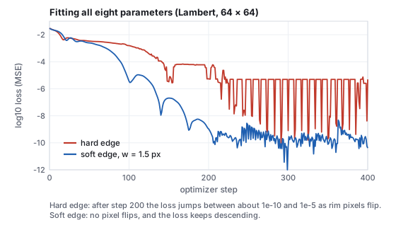
The update is the gradient descent of the networks chapter, usually with Adam (same chapter) because parameters with different units (an albedo in [0, 1], an angle in radians, a radius) need different step sizes and Adam normalizes each by its own gradient history.
| step | 0 | 10 | 50 | 100 | 200 | 300 |
|---|---|---|---|---|---|---|
| loss, hard edge | 0.0304 | 0.0156 | 0.00337 | 0.00157 | 5.4×10⁻⁶ | 8.0×10⁻¹⁰ |
| loss, soft edge (Section 7) | 0.0297 | 0.0185 | 0.00249 | 3.6×10⁻⁶ | 1.1×10⁻⁹ | 5.2×10⁻¹¹ |

4 · Automatic differentiation: forward and reverse
A renderer is a long composition of elementary operations. Automatic differentiation (AD) applies the chain rule to that composition exactly, operation by operation; it is neither symbolic differentiation (which builds an expression) nor finite differences (which perturb inputs and suffer truncation and rounding error). Wengert (1964) described the forward mode; Linnainmaa (1976) the reverse mode, which reached machine learning as backpropagation (Rumelhart, Hinton and Williams 1986). Baydin et al. (2018) survey both, and Griewank and Walther’s Evaluating Derivatives is the reference.
| \(u\) | \(s\) | \(P\) | \(L\) | |
|---|---|---|---|---|
| forward, seed \(\dot\rho = 1\) | 0 | 0 | \(s = 0.9416\) | \(2(P-T)\dot P = -0.4316\) |
| forward, seed \(\dot\phi = 1\) | 0.3368 | 0.3368 | \(\rho\dot s = 0.1684\) | \(-0.0772\) |
The course renderer writes its reverse pass by hand: for each pixel it evaluates the color, then applies the chain rule backward through that pixel’s coverage, normal, Lambert and Blinn–Phong terms, accumulating eight adjoints. The function lossAndGrad in lib/core/inverse-render.js is about sixty lines; the test file checks every component against central finite differences (next section).
5 · Differentiating shading and lighting
Away from edges, a pixel’s color is a smooth function of the parameters, and its derivatives follow from the shading model of the illumination chapter:
- \(\partial P/\partial\rho_c = 0.08 + 0.9941 = 1.0741\), so this pixel adds \(2(0.5370 - 0.2004) \cdot 1.0741 / 12{,}288 = 5.89\times10^{-5}\) to \(\partial L/\partial\rho_R\): lower the red albedo;
- \(\partial(\mathbf{n}\cdot\mathbf{l})/\partial\phi_a = \mathbf{n}\cdot(0.8776, 0, 0.4794) = -0.1064\), and the three channels together add \((0.6733 + 0.9091 + 0.9798)\cdot 0.5 \cdot (-0.1064) / 12{,}288 = -1.11\times10^{-5}\) to \(\partial L/\partial\phi_a\): a negative derivative, so descent increases the azimuth, swinging the light toward its true side and darkening this pixel.
The \(\max(0, \cdot)\) is already a mild problem: its derivative jumps from 0 to 1 at the terminator, and a point in shadow passes no gradient to the light at all. A pixel that should be lit but is in the current shadow cannot pull the light toward itself; only lit pixels vote. Global effects add more of the same: a shadow’s edge, a reflection’s boundary and a refraction all move with the parameters, and each is a discontinuity in the integrand.
6 · The visibility discontinuity
A pixel’s true value is an integral of the scene’s radiance over the pixel’s area (the antialiasing chapter). When an edge crosses the pixel, the integrand is discontinuous, and the discontinuity moves with the parameters.
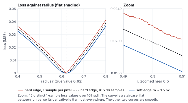
Sampling a pixel at fixed points and differentiating each sample captures the interior term only. A sample is either on one side of the edge or the other; an infinitesimal change of \(\theta\) moves no sample across, so its derivative is the interior one, and the boundary term is lost. This is not a numerical accident: Monte Carlo estimators of the pixel integral differentiated sample by sample are biased estimators of its derivative.
| pixel model | loss at \(r = 0.5\) | \(\partial L/\partial r\) |
|---|---|---|
| hard edge, 1 sample at each pixel center, analytic | 0.02194 | 0 (central differences, \(h = 10^{-6}\): also 0) |
| hard edge, 16 × 16 samples, central differences (\(h = 10^{-3}\)) | 0.01982 | −0.1635 |
| soft edge, \(w = 1.5\) pixels, analytic | 0.01785 | −0.1650, all of it from the rim |
7 · Four answers to the edge problem
Each family restores the boundary term in a different way.
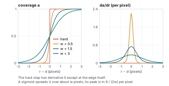
| \(r - d\) (pixels) | −1 | −0.5 | 0 | 0.5 | 1 |
|---|---|---|---|---|---|
| coverage \(a\) | 0.0507 | 0.1877 | 0.5 | 0.8123 | 0.9493 |
Rasterization-based systems in production combine these ideas: nvdiffrast (Laine et al. 2020) keeps a hard, fast rasterizer and adds an analytic antialiasing pass whose derivative supplies the silhouette gradient, and PyTorch3D (Ravi et al. 2020) implements a soft rasterizer for meshes and point clouds.
8 · Differentiable path tracers
A naive reverse-mode differentiation of a path tracer must store every intermediate value of every path for the backward pass. Assume 50 stored floats per path vertex: a 512 × 512 image at 64 samples per pixel and 6 bounces records \(512^2 \cdot 64 \cdot 6 \cdot 50 \cdot 4\) bytes, 20.1 GB, for one gradient. The systems below exist to avoid that.
Monte Carlo adds a statistical problem. A gradient estimated from the same random samples as the forward value it multiplies is biased (the product of two correlated estimates is not the estimate of the product), so these systems decorrelate, using independent samples for the two factors. Zeltner et al. (2021) analyze the estimators and their variance; the practical rule is that a differentiable path tracer needs far fewer samples per iteration than a final render, because an optimizer averages noisy gradients over steps, but its estimators must be unbiased or the average converges to the wrong answer.
9 · What can be recovered
| unknown | representation | typical method | typical difficulty |
|---|---|---|---|
| materials | BRDF parameters (albedo, roughness, metalness) per object, or textures | known geometry and lights; gradient of the image loss through the BRDF (the light-transport chapter) | albedo against light intensity; specular highlights cover few pixels |
| lighting | environment map, area lights | inverse path tracing with known geometry (Azinović et al. 2019 recover materials and emitters of a room jointly) | only low frequencies recoverable from diffuse surfaces |
| geometry | mesh vertices, signed distance functions | silhouette-aware gradients; Laplacian preconditioning (Nicolet, Jacobson and Jakob 2021); SDF gradients (Vicini, Speierer and Jakob 2022) | visibility; self-intersections and tangling under raw vertex gradients |
| all three | mesh + materials + environment light | nvdiffrec (Munkberg et al. 2022): differentiable rasterization end to end, exportable to a game engine | the ambiguities of Section 2 at once |
| volumes | density and albedo grids | differentiable volumetric path tracing (Mitsuba 2’s volume examples) | memory; many scattering events per path |
Geometry is the hardest case for a reason visible in the course renderer: raw vertex gradients are large near silhouettes and noisy, and a step that follows them moves vertices independently and tangles the mesh. Nicolet et al. precondition the step by \((I + \lambda L)^{-1}\) with \(L\) the mesh Laplacian (the meshes chapter), which spreads each vertex’s update over its neighbors and allows large, smooth steps.
10 · NeRF and splatting as inverse rendering
The learned scenes of the learned-scenes chapter are inverse rendering with a particular choice of representation and renderer, chosen so that the visibility problem does not arise.
- NeRF renders by the volume integral, in which occlusion is a product of transmittances \(T_i = \prod_{j<i}(1-\alpha_j)\) and every quantity is a smooth function of the densities. There is no edge to sample: a surface is a steep but differentiable rise in density.
- 3D Gaussian splatting renders by sorted alpha blending of Gaussians, each with a smooth footprint. Coverage is the Gaussian’s value, a soft edge by construction; only the sort order is discrete, and it changes rarely enough that its gradient is ignored.
Both invert for radiance, not for materials and lights: the scene they recover reproduces the photographs from new viewpoints but bakes in the capture’s lighting, which is why they cannot be relit without a further decomposition (the relighting question of the generative-3D lecture). Physically based inverse rendering recovers the factors at the cost of the ambiguities of Section 2; learned scenes avoid the ambiguities by not factoring.
11 · Regularization and priors
Barron and Malik (2015) recovered shape, illumination and reflectance from a single image by combining many such hand-built priors (smooth shape, sparse reflectance changes, natural illumination). Learned priors replace the hand-built ones: a network trained on many scenes predicts parameters directly or initializes the optimization, and a diffusion model can act as the prior itself, scoring how plausible a rendered view looks. Score distillation (DreamFusion, Poole et al. 2022; the diffusion chapter) is this idea taken to its limit: no photograph at all, only the prior, pushed through a differentiable renderer.
12 · Open problems
- Global-illumination gradients. Boundary terms from shadows, reflections and caustics deep in a path are expensive to find and high in variance; unbiased path-space estimators exist, but their cost per useful gradient is still far above that of a forward render.
- Noise. Gradient variance slows optimization and correlated estimators bias it; how many samples to spend on the forward value against the gradient, and how to share them across iterations, is open.
- Local minima. The loss of an image is not convex in geometry or light: a shape that must move further than its silhouette’s width sees no gradient pulling it there, and the explaining-away of Section 6 is a minimum the optimizer is content with. Coarse-to-fine schedules, wide soft edges at first, and learned initializations are the current remedies.
- Real capture. A photograph is not a render: the camera has an unknown response curve, white balance, lens distortion, vignetting, motion blur and noise, and the scene has interreflections and lights outside the frame. Every one must be modeled or calibrated, or the optimizer absorbs it into the parameters.
- From the offering’s webroot, run the gradient checks of the course renderer:
node --test lib/tests/inverse-render.test.mjs. Expected, at the end:ℹ tests 10,ℹ pass 10,ℹ fail 0. The first six tests compare all eight analytic derivatives with central differences under flat, Lambert and Blinn–Phong shading, hard and soft edges. - Measure the silhouette gradient of Section 6 yourself (save as
edge.mjsin the webroot):import { TRUE_PARAMS, render, lossAndGrad } from './lib/core/inverse-render.js'; const p = TRUE_PARAMS.slice(); p[5] = 0.5; for (const edge of ['hard', 'soft']) { const o = { n: 64, edge, shading: 'flat', w: 1.5 }; const g = lossAndGrad(p, render(TRUE_PARAMS, o), o); console.log(edge, 'loss', g.loss.toFixed(5), 'dL/dr', g.grad[5].toFixed(4)); }Expected:hard loss 0.02194 dL/dr 0.0000andsoft loss 0.01785 dL/dr -0.1650. - Run the whole fit with a soft edge:
import { TRUE_PARAMS, START_PARAMS, render, makeFit } from './lib/core/inverse-render.js';
const o = { n: 64, edge: 'soft', shading: 'lambert', w: 1.5 };
const fit = makeFit({ start: START_PARAMS, target: render(TRUE_PARAMS, o), opts: o, free: Array(8).fill(true) });
for (let i = 1; i <= 300; i++) { const r = fit.step(); if (i % 100 === 0) console.log(i, r.loss.toExponential(2), fit.p.map((v) => v.toFixed(3)).join(' ')); }
Expected (the loss printed is the one measured before stepi’s update):100 5.11e-6 0.842 0.349 0.200 0.700 0.450 0.620 0.081 -0.060 200 1.20e-9 0.850 0.350 0.200 0.700 0.450 0.620 0.080 -0.060 300 5.48e-13 0.850 0.350 0.200 0.700 0.450 0.620 0.080 -0.060
- In the inverse-render demo, choose flat, hard, optimize radius, and press play: the readout
dL/dr rim, inshows0, 0and the radius stays at 0.42. Switch the edge to soft: the bottom-right panel lights up red along the rim and the radius walks to 0.62.
13 · The papers
| Year | Paper | What it added |
|---|---|---|
| 1964 | Wengert, “A simple automatic derivative evaluation program,” CACM, doi:10.1145/355586.364791 | forward-mode AD |
| 1976 | Linnainmaa, “Taylor expansion of the accumulated rounding error,” BIT, doi:10.1007/BF01931367 | reverse-mode AD |
| 1986 | Rumelhart, Hinton & Williams, “Learning representations by back-propagating errors,” Nature, doi:10.1038/323533a0 | reverse mode as backpropagation |
| 1999 | Blanz & Vetter, “A morphable model for the synthesis of 3D faces,” SIGGRAPH, doi:10.1145/311535.311556 | analysis by synthesis of faces |
| 2001 | Ramamoorthi & Hanrahan, “A signal-processing framework for inverse rendering,” SIGGRAPH, doi:10.1145/383259.383271 | what lighting and reflectance can be recovered |
| 2008 | Griewank & Walther, Evaluating Derivatives, 2nd ed., SIAM, doi:10.1137/1.9780898717761 | the reference on AD |
| 2014 | Loper & Black, “OpenDR: an approximate differentiable renderer,” ECCV, doi:10.1007/978-3-319-10584-0_11 | a general differentiable rasterizer |
| 2015 | Barron & Malik, “Shape, illumination, and reflectance from shading,” TPAMI, doi:10.1109/TPAMI.2014.2377712 | inverse rendering from one image with priors |
| 2018 | Baydin, Pearlmutter, Radul & Siskind, “Automatic differentiation in machine learning: a survey,” JMLR, arXiv:1502.05767 | survey of AD |
| 2018 | Kato, Ushiku & Harada, “Neural 3D Mesh Renderer,” CVPR, doi:10.1109/CVPR.2018.00411 | approximate rasterization gradients |
| 2018 | Li, Aittala, Durand & Lehtinen, “Differentiable Monte Carlo ray tracing through edge sampling,” TOG, doi:10.1145/3272127.3275109 | unbiased edge sampling |
| 2019 | Liu, Li, Chen & Li, “Soft Rasterizer,” ICCV, doi:10.1109/ICCV.2019.00780 | probabilistic coverage and aggregation |
| 2019 | Loubet, Holzschuch & Jakob, “Reparameterizing discontinuous integrands for differentiable rendering,” TOG, doi:10.1145/3355089.3356510 | reparameterization |
| 2019 | Nimier-David, Vicini, Zeltner & Jakob, “Mitsuba 2: a retargetable forward and inverse renderer,” TOG, doi:10.1145/3355089.3356498 | one renderer, many variants, differentiable |
| 2019 | Azinović, Li, Kaplanyan & Nießner, “Inverse path tracing for joint material and lighting estimation,” CVPR, arXiv:1903.07145 | materials and emitters of a room |
| 2020 | Zhang, Miller, Yan, Gkioulekas & Zhao, “Path-space differentiable rendering,” TOG, doi:10.1145/3386569.3392383 | boundary terms in path space |
| 2020 | Nimier-David, Speierer, Ruiz & Jakob, “Radiative backpropagation,” TOG, doi:10.1145/3386569.3392406 | the backward pass as light transport |
| 2020 | Bangaru, Li & Durand, “Unbiased warped-area sampling for differentiable rendering,” TOG, doi:10.1145/3414685.3417833 | unbiased reparameterization |
| 2020 | Laine, Hellsten, Karras, Seol, Lehtinen & Aila, “Modular primitives for high-performance differentiable rendering,” TOG, doi:10.1145/3414685.3417861 | nvdiffrast |
| 2020 | Ravi et al., “Accelerating 3D deep learning with PyTorch3D,” arXiv:2007.08501 | a soft mesh and point rasterizer in a library |
| 2020 | Mildenhall et al., “NeRF,” arXiv:2003.08934 | a scene as a radiance field, fitted through the volume integral |
| 2021 | Vicini, Speierer & Jakob, “Path replay backpropagation,” TOG, doi:10.1145/3450626.3459804 | linear-time backward pass |
| 2021 | Zeltner, Speierer, Georgiev & Jakob, “Monte Carlo estimators for differential light transport,” TOG, doi:10.1145/3450626.3459807 | gradient estimators and their variance |
| 2021 | Nicolet, Jacobson & Jakob, “Large steps in inverse rendering of geometry,” TOG, doi:10.1145/3478513.3480501 | Laplacian preconditioning for meshes |
| 2022 | Jakob, Speierer, Roussel & Vicini, “Dr.Jit: a just-in-time compiler for differentiable rendering,” TOG, doi:10.1145/3528223.3530099 | the compiler under Mitsuba 3 |
| 2022 | Vicini, Speierer & Jakob, “Differentiable signed distance function rendering,” TOG, doi:10.1145/3528223.3530139 | SDF geometry from images |
| 2022 | Munkberg et al., “Extracting triangular 3D models, materials, and lighting from images,” CVPR, arXiv:2111.12503 | nvdiffrec |
| 2022 | Poole, Jain, Barron & Mildenhall, “DreamFusion,” arXiv:2209.14988 | a diffusion model as the only prior |
| 2023 | Kerbl, Kopanas, Leimkühler & Drettakis, “3D Gaussian splatting for real-time radiance field rendering,” TOG, doi:10.1145/3592433 | soft primitives, sorted blending |
14 · Exercises
Solution
\(2(P_G - T_G) = 2(0.5370 - 0.0825) = 0.9091\); times \(\partial P/\partial\rho_G = 1.0741\), divided by 12,288: \(7.95\times10^{-5}\). Positive, so descent lowers the green albedo, toward the true 0.35.Solution
Forward mode: one pass per input, \(3 \cdot 1024^2 = 3{,}145{,}728\) passes. Reverse mode: one forward and one backward pass, because there is one output. It pays in memory: the tape of intermediate values from the forward pass (or, in radiative backpropagation, a second transport simulation instead of a tape).Solution
\(I(t) = 0.8t + 0.1(1 - t) = 0.1 + 0.7t\), so \(dI/dt = 0.7 = f_{\text{in}} - f_{\text{out}}\): all boundary term, since \(\partial f/\partial t = 0\) away from the edge. The center sample at \(x = 0.5\) reads 0.1 for every \(t\) near 0.3, so its derivative is 0. The sample changes only when \(t\) crosses 0.5, by a jump of 0.7, which no derivative sees.Solution
\(s = 1.5/(2\ln 9) = 0.3413\) pixels, \(a = \sigma(0.5/0.3413) = \sigma(1.4648) = 0.8123\). \(da/dr = a(1-a)/s = 0.8123 \cdot 0.1877 / 0.3413 = 0.4467\) per pixel, against the peak 0.732 at the rim itself.Solution
With \(k_a = 0\), \(S = \rho E \max(0, \mathbf{n}\cdot\mathbf{l})\), a function of the product. With \(k_a > 0\), \(S = \rho k_a + \rho E \max(0,\cdot)\): the shadowed side reads \(\rho k_a\) alone, which fixes \(\rho\) if \(k_a\) is known. In a photograph the ambient light is itself an unknown (it is the rest of the environment), so it is one more factor multiplying \(\rho\), and the tie returns.Solution
\(1024^2 \cdot 16 \cdot 4 \cdot 50 \cdot 4 = 13{,}421{,}772{,}800\) bytes, 13.4 GB, more than many GPUs hold, for one gradient. Radiative backpropagation needs the memory of a forward render.Solution
\(s = 0.6/0.4667 = 1.286\), \(E = 1/s = 0.778\), albedo \((1.029, 0.514, 0.257)\). The red albedo exceeds 1, which is physically impossible; a box constraint \(\rho \le 1\) (the course optimizer clamps albedos to [0, 1]) would stop at \(s = 1.25\), \(E = 0.8\). Priors and constraints interact.Solution
Nothing: the derivative of \(\max(0, u)\) at \(u < 0\) is 0, so the pixel passes no gradient to the light, however large its error. The light is pulled only by pixels that are lit now. A fit starting with the light behind the object sees a thin lit crescent and moves slowly or not at all; the albedo, which still receives the ambient term’s gradient, may darken to compensate. Coarse-to-fine schedules and multiple starts address this.lib/core/inverse-render.js, render the flat disk with a hard edge at 16 × 16 samples per pixel (spp: 16) and estimate \(\partial L/\partial r\) at \(r = 0.5\) by central differences with \(h = 10^{-3}\). Compare with the soft edge’s analytic value. Then try \(h = 10^{-6}\) and explain the result.
Solution
import { TRUE_PARAMS, render, mse } from './lib/core/inverse-render.js';
const o = { n: 64, edge: 'hard', shading: 'flat', spp: 16 };
const T = render(TRUE_PARAMS, o);
const at = (r) => { const p = TRUE_PARAMS.slice(); p[5] = r; return mse(render(p, o), T); };
for (const h of [1e-3, 1e-6]) console.log(h, ((at(0.5 + h) - at(0.5 - h)) / (2 * h)).toFixed(4));
At \(h = 10^{-3}\) the estimate is \(-0.1635\), against the soft edge’s \(-0.1650\). At \(h = 10^{-6}\) it reads \(-0.1069\); at \(2\times10^{-6}\), \(-0.0534\); at \(5\times10^{-7}\), 0. The perturbation moves the rim by far less than the subsample spacing (1/16 of a pixel is \(1.95\times10^{-3}\)), so it crosses one subsample, or two, or none, and the quotient is the size of those few jumps divided by \(2h\), not a derivative. Supersampling only pushes the staircase to a finer scale; the step must be larger than the subsample spacing for the quotient to mean anything.