This chapter links to the course’s interactive demos and to original papers on the open web, and it uses MathJax for its formulas. Read it through the course website (or download the file and open it in a browser); a Canvas inline preview will reach neither the demos nor the math. All chapters.

Neural Networks and Embeddings

Frank Rosenblatt demonstrated the perceptron in 1958; the Mark I Perceptron's camera was a 20 × 20 grid of photocells, a 400-pixel image. Rosenblatt, Psychological Review, 1958; Cornell Aeronautical Laboratory, Mark I Perceptron, 1960

Three ideas underlie every model in the chapters that follow: a neural network is a function whose weights are set by examples; an embedding is a learned vector that stands for a concept, placed so that similar concepts are near; and an encoder and a decoder move between things and their embeddings, with two encoders trained side by side making words and pictures one coordinate system. This chapter states each idea, runs the smallest possible example of it by hand, and shows the same thing computed at full size from the course’s own trained network. Between the ideas it supplies what a working model needs: the activation functions and their derivatives, backpropagation through more than one hidden layer, the optimizers that replace plain gradient descent, the overfitting that a held-out set exposes and weight decay tames, and the two layer types, convolution and attention, that image and text models are built from.

Contents
  1. A network is a function
  2. Training is gradient descent
  3. Backpropagation through two hidden layers
  4. Optimizers: momentum and Adam
  5. What a trained network is good for, and overfitting
  6. Two more layers: convolution and attention
  7. Embeddings
  8. Encoders, decoders, and one shared space
  9. Coordinate networks
  10. The papers
  11. Exercises

1 · A network is a function

Definition (neural network) A neural network is a function \(f_\theta : \mathbb{R}^{n} \to \mathbb{R}^{m}\) built from alternating linear maps and fixed nonlinearities, whose behavior is set by a vector of weights \(\theta\). The two-layer perceptron of the lecture’s approximator exhibit is \[ f_\theta(x) \;=\; b_2 + \sum_{h=1}^{H} w^{(2)}_h \,\tanh\!\big(w^{(1)}_h x + b^{(1)}_h\big), \qquad \theta = (w^{(1)}, b^{(1)}, w^{(2)}, b_2) \in \mathbb{R}^{3H+1}. \]
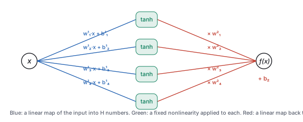
Diagram of a one-input perceptron: the input x fans out through four blue linear edges into four tanh units, whose outputs are scaled by red weights and summed with a bias into f(x).
The perceptron as a wiring diagram, \(H = 4\). Read left to right: the input is multiplied by \(H\) weights and offset by \(H\) biases (blue), each result is squashed by \(\tanh\) (green), and the \(H\) squashed numbers are combined by a second linear map (red). Nothing else happens. A “deep” network repeats the middle two stages several times, with vectors in place of single numbers.

There is no mystery in evaluating one. The point of the next example is that you can do it with a pocket calculator, and that every larger network is the same arithmetic with more rows.

Worked example (a forward pass by hand) Take \(H = 2\) with weights \(w^{(1)} = (1.0, -1.0)\), \(b^{(1)} = (0.5, 0.5)\), \(w^{(2)} = (0.8, -0.6)\), \(b_2 = 0.1\), and the input \(x = 0.4\).
pre-activations\(z_1 = 1.0\times0.4 + 0.5 = 0.9\),    \(z_2 = -1.0\times0.4 + 0.5 = 0.1\)
activations\(a_1 = \tanh 0.9 = 0.7163\),    \(a_2 = \tanh 0.1 = 0.0997\)
output\(f = 0.1 + 0.8\times0.7163 - 0.6\times0.0997 = 0.1 + 0.5730 - 0.0598 = 0.6132\)
Seven weights, four multiplications, three additions, two table lookups. The digit-drawing network of the diffusion chapter has a million weights and its forward pass is about a million multiply-adds; it is this table with 512 rows per stage and four stages.

1.1 The nonlinearity

Without the squashing step a network of any depth is a single linear map, because a composition of linear maps is linear; the nonlinearity is what makes depth do anything. Which one is a choice, and the choices in use differ in what their derivative does, which Section 2 makes matter.
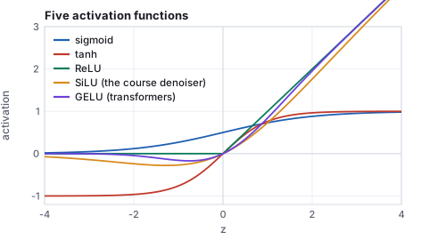
Five activation curves over z from minus 4 to 4: sigmoid rising from 0 to 1, tanh from minus 1 to 1, ReLU flat at zero then a line of slope one, SiLU dipping slightly below zero before joining ReLU, and GELU between them.
Five activations. The saturating pair (sigmoid, tanh) have derivatives that vanish for large inputs; the rectifier family (ReLU, SiLU, GELU) keep a slope of 1 on the positive side. The course’s denoiser uses SiLU.
name\(\sigma(z)\)\(\sigma'(z)\)value at \(z = 0.9\)slope at \(0.9\)where it is used
sigmoid\(1/(1 + e^{-z})\)\(\sigma(1 - \sigma)\)0.7110.206probabilities; gates
tanh\((e^{z} - e^{-z})/(e^{z} + e^{-z})\)\(1 - \tanh^2 z\)0.7160.487the perceptron above; small networks
ReLU\(\max(0, z)\)\(0\) or \(1\)0.9001most deep networks since 2012
SiLU\(z\,\sigma(z)\)\(\sigma(z)\,(1 + z(1 - \sigma(z)))\)0.6400.896the course denoiser; diffusion U-Nets
GELU\(z\,\Phi(z)\), \(\Phi\) the normal CDFnumerical0.734near 0.9transformers

The saturating functions were the original choice and are still right for a small network like the perceptron; in a deep one their vanishing derivative multiplies through the layers and the early weights stop learning (the vanishing gradient). The rectifiers keep the gradient alive on their active side, and their smooth variants keep it alive everywhere.

2 · Training is gradient descent

Training is not programming. Given examples \((x_i, y_i)\), define a loss such as the mean squared error \(\mathcal{L}(\theta) = \frac{1}{N}\sum_i (f_\theta(x_i) - y_i)^2\), and repeat two steps: compute the gradient \(\nabla_\theta \mathcal{L}\), the direction in weight space that increases the loss fastest, and move every weight a little the other way,

\[ \theta \;\leftarrow\; \theta - \eta\, \nabla_\theta \mathcal{L}(\theta), \]

with a small learning rate \(\eta\). The gradient is computed by the chain rule, organized so that every weight’s derivative is obtained in one backward sweep through the diagram; that organization is backpropagation (Rumelhart, Hinton & Williams 1986). For the perceptron the four derivatives are short enough to write down:

\[ \begin{gathered} \frac{\partial \mathcal{L}}{\partial b_2} = \delta, \qquad \frac{\partial \mathcal{L}}{\partial w^{(2)}_h} = \delta\, a_h, \qquad \delta = 2\,(f - y), \\[4pt] \frac{\partial \mathcal{L}}{\partial w^{(1)}_h} = \delta\, w^{(2)}_h (1 - a_h^2)\, x, \qquad \frac{\partial \mathcal{L}}{\partial b^{(1)}_h} = \delta\, w^{(2)}_h (1 - a_h^2), \end{gathered} \]

for a single example (average over the batch for more), using \(\tanh' = 1 - \tanh^2\). Notice how the backward sweep reuses the forward one: the \(a_h\) were already computed, and \(\delta\) is one number passed back through the red edges, then through the green boxes, to reach the blue edges.

Worked example (one gradient step by hand) Continue the example above with the target \(y = 0.3\) and \(\eta = 0.1\). The error is \(f - y = 0.3132\), the loss \(0.3132^2 = 0.0981\), and \(\delta = 0.6265\).
\(\partial/\partial b_2\)\(0.6265\)
\(\partial/\partial w^{(2)}\)\(0.6265\times(0.7163,\; 0.0997) = (0.4487,\; 0.0624)\)
\(1 - a_h^2\)\((1 - 0.5131,\; 1 - 0.0099) = (0.4869,\; 0.9901)\)
\(\partial/\partial b^{(1)}\)\(0.6265\times(0.8\times0.4869,\; -0.6\times0.9901) = (0.2440,\; -0.3722)\)
\(\partial/\partial w^{(1)}\)the previous row times \(x = 0.4\): \((0.0976,\; -0.1489)\)
Step every weight against its gradient, \(\theta \leftarrow \theta - 0.1\,\nabla\): \(w^{(1)} = (0.9902, -0.9851)\), \(b^{(1)} = (0.4756, 0.5372)\), \(w^{(2)} = (0.7551, -0.6062)\), \(b_2 = 0.0374\). Rerun the forward pass with the new weights: \(f = 0.4814\), loss \(0.0329\), down from \(0.0981\). One step took the output a third of the way to the target; the sign of every change was decided by the chain rule, not by anyone looking at the problem. Repeat a few thousand times over a few thousand examples and that is all training is.
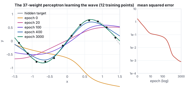
Left: twelve training points on a hidden sine-like curve, with the perceptron's curve drawn at epochs 0, 20, 100, 400 and 3000 bending progressively onto the points. Right: the mean squared error falling from about 1.7 to below 0.001 on a log-log plot.
The approximator exhibit, computed offline by the same library the demo runs: \(H = 12\) (37 weights), full-batch gradient descent on 12 points of a hidden wave, \(\eta = 0.05\). The random-weight curve (orange) has nothing to do with the data; by epoch 20 it has found the general slope, by 400 the shape, by 3000 it passes through every point and follows the hidden curve between them. Loss: 1.73, 0.105, 0.069, 0.0084, 0.0008.
See it live A network that learns: the same 37-weight perceptron trained in your browser. Drag epochs from 0 and watch the curve bend a few steps per frame while the loss plot falls; try 2 hidden units (it cannot bend enough) and 40 (it fits a step with a smooth ramp).
Pitfall The learning rate is the one number that can make training fail outright. On the wave fit with \(H = 12\), 300 epochs at \(\eta = 0.05\) reach a loss of 0.019; at \(\eta = 0.3\) and at \(\eta = 1.0\) the loss is not a number within 300 epochs. A step that overshoots the valley lands higher on the far wall, the next gradient is larger, the step larger still, and the weights blow up in a few dozen iterations. The symptom is a loss that rises instead of falls, or becomes NaN; the cure is a smaller rate, a schedule that decays it, or the optimizers of Section 4, whose normalization bounds each step regardless of the gradient’s size.

3 · Backpropagation through two hidden layers

The perceptron has one hidden layer, and its gradient has a special form. The general form is one rule applied once per layer: the error signal \(\boldsymbol\delta^{(k)} = \partial\mathcal{L}/\partial\mathbf{z}^{(k)}\) at layer \(k\) is the error signal of the layer above, multiplied by that layer’s weights transposed, times the derivative of the activation, \[ \boldsymbol\delta^{(k)} \;=\; \big(W^{(k+1)\top}\,\boldsymbol\delta^{(k+1)}\big)\odot \sigma'(\mathbf{z}^{(k)}), \qquad \frac{\partial\mathcal{L}}{\partial W^{(k)}} = \boldsymbol\delta^{(k)}\,\mathbf{a}^{(k-1)\top}, \quad \frac{\partial\mathcal{L}}{\partial \mathbf{b}^{(k)}} = \boldsymbol\delta^{(k)}, \] with \(\odot\) the elementwise product and \(\mathbf{a}^{(k-1)}\) the activations feeding the layer. Each weight’s gradient is the error arriving at its output times the activation at its input. The forward pass stores every \(\mathbf{a}\); the backward pass is one matrix multiply per layer.

Worked example (a 1–2–2–1 network) Keep the first layer of Section 1 (\(W^{(1)} = (1.0, -1.0)\), \(\mathbf{b}^{(1)} = (0.5, 0.5)\)), add a second hidden layer \(W^{(2)} = \begin{pmatrix} 0.6 & -0.4 \\ 0.3 & 0.9 \end{pmatrix}\), \(\mathbf{b}^{(2)} = (0, -0.2)\), and an output \(\mathbf{w}^{(3)} = (0.8, -0.6)\), \(b^{(3)} = 0.1\); \(\tanh\) everywhere; \(x = 0.4\), \(y = 0.3\), \(\eta = 0.1\).
forward, layer 1\(\mathbf{z}^{(1)} = (0.9, 0.1)\), \(\mathbf{a}^{(1)} = (0.7163, 0.0997)\), as before
forward, layer 2\(z^{(2)}_1 = 0.6(0.7163) - 0.4(0.0997) + 0 = 0.3899\), \(z^{(2)}_2 = 0.3(0.7163) + 0.9(0.0997) - 0.2 = 0.1046\); \(\mathbf{a}^{(2)} = (0.3713, 0.1042)\)
forward, output\(f = 0.1 + 0.8(0.3713) - 0.6(0.1042) = 0.3345\); loss \((0.0345)^2 = 0.0012\)
\(\delta^{(3)}\)\(2(f - y) = 0.0690\); gradients \(\partial/\partial b^{(3)} = 0.0690\), \(\partial/\partial\mathbf{w}^{(3)} = 0.0690\,\mathbf{a}^{(2)} = (0.0256, 0.0072)\)
\(\boldsymbol\delta^{(2)}\)\(\delta^{(3)}\,\mathbf{w}^{(3)}\odot(1 - \mathbf{a}^{(2)2}) = 0.0690\,(0.8, -0.6)\odot(0.8621, 0.9891) = (0.0476, -0.0410)\)
\(\partial/\partial W^{(2)}\)\(\boldsymbol\delta^{(2)}\mathbf{a}^{(1)\top} = \begin{pmatrix} 0.0341 & 0.0047 \\ -0.0293 & -0.0041 \end{pmatrix}\); \(\partial/\partial\mathbf{b}^{(2)} = (0.0476, -0.0410)\)
\(\boldsymbol\delta^{(1)}\)\(W^{(2)\top}\boldsymbol\delta^{(2)} = (0.6(0.0476) + 0.3(-0.0410),\; -0.4(0.0476) + 0.9(-0.0410)) = (0.0163, -0.0559)\), times \((1 - \mathbf{a}^{(1)2}) = (0.4869, 0.9901)\): \((0.0079, -0.0553)\)
\(\partial/\partial W^{(1)}\)\(\boldsymbol\delta^{(1)}\,x = (0.0032, -0.0221)\); \(\partial/\partial\mathbf{b}^{(1)} = (0.0079, -0.0553)\)
after the step\(f = 0.3126\), loss \(0.0002\): down by a factor of six
Thirteen weights, one backward sweep, and the deepest weights got the smallest gradients: \(\boldsymbol\delta\) was multiplied by \(w^{(3)}\), then by \(W^{(2)}\), and at each layer by a \(\tanh'\) below 1. Ten layers of that and the first layer would barely move, which is the vanishing gradient of Section 1 seen in numbers, and the reason for the rectifiers, for careful initialization, and for the skip connections that let \(\boldsymbol\delta\) bypass layers in every deep network built since 2015.

Automatic differentiation (PyTorch’s backward()) does exactly this sweep for any composition of operations, recording the forward pass as a graph and walking it in reverse; nobody writes the gradient of a modern network by hand. The point of writing this one is that there is nothing else in the box.

4 · Optimizers: momentum and Adam

Plain gradient descent has two faults that the loss curve of Section 2 shows: it takes tiny steps where the loss surface is flat, and it oscillates where the surface is a narrow valley, because the gradient points across the valley more than along it. Two amendments fix both, and one of them is the default of every training script.
Definition (momentum, Adam) Momentum keeps a running velocity, \(\mathbf{v} \leftarrow \beta\mathbf{v} + \mathbf{g}\), \(\theta \leftarrow \theta - \eta\mathbf{v}\), with \(\beta \approx 0.9\): gradients that agree from step to step add up (a rolling ball), gradients that alternate cancel. Adam (Kingma and Ba, 2015) keeps two running averages, of the gradient and of its square, \[ \mathbf{m} \leftarrow \beta_1\mathbf{m} + (1 - \beta_1)\mathbf{g}, \qquad \mathbf{v} \leftarrow \beta_2\mathbf{v} + (1 - \beta_2)\mathbf{g}^2, \qquad \theta \leftarrow \theta - \eta\,\frac{\hat{\mathbf{m}}}{\sqrt{\hat{\mathbf{v}}} + \epsilon}, \] with \(\hat{\mathbf{m}} = \mathbf{m}/(1 - \beta_1^t)\), \(\hat{\mathbf{v}} = \mathbf{v}/(1 - \beta_2^t)\) correcting the averages’ bias toward zero at the start, and defaults \(\beta_1 = 0.9\), \(\beta_2 = 0.999\), \(\epsilon = 10^{-8}\). Each weight gets its own step size, the learning rate divided by the typical size of that weight’s gradient.
Worked example (the first Adam step) Apply Adam with \(\eta = 0.01\) to the seven gradients of Section 2, \(\mathbf{g} = (0.0976, -0.1489, 0.2440, -0.3722, 0.4487, 0.0624, 0.6265)\). At \(t = 1\), \(\mathbf{m} = 0.1\mathbf{g}\) and \(\hat{\mathbf{m}} = \mathbf{g}\); \(\mathbf{v} = 0.001\mathbf{g}^2\) and \(\hat{\mathbf{v}} = \mathbf{g}^2\); so every update is \(\eta\,\mathbf{g}/|\mathbf{g}| = \pm0.01\). The weight with gradient 0.0624 and the weight with gradient 0.6265 both move by 0.01. Gradient descent would have moved them by 0.006 and 0.063 at the same \(\eta\). Adam’s first step is a step of length \(\eta\) along the sign of the gradient in every coordinate; later steps shrink for coordinates whose gradient is noisy (large \(\hat{\mathbf{v}}\) relative to \(\hat{\mathbf{m}}^2\)) and stay near \(\eta\) for coordinates whose gradient is consistent. That is why the pitfall of Section 2 does not apply to it in the same way: a step cannot exceed about \(\eta\) per coordinate, whatever the gradient.
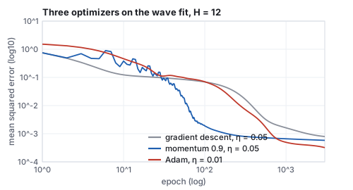
Three loss curves on a log-log plot over 3000 epochs of the wave fit: plain gradient descent in gray falls slowly to about 0.001, momentum in blue drops steeply past epoch 100 and oscillates early, Adam in red plateaus then falls to 0.0003 by 3000.
The wave fit of Section 2 three ways, same initialization, same 12 points. Mean squared error at epochs 100, 300, 1000, 3000: gradient descent 0.069, 0.019, 0.0016, 0.0008; momentum 0.0019, 0.0008, 0.0007, 0.0006; Adam 0.070, 0.008, 0.0005, 0.0003. Momentum is fastest here (a smooth, low-dimensional problem); Adam ends lowest.

On a large network trained on minibatches, whose gradients are noisy estimates, Adam’s per-weight normalization is what makes one learning rate work across layers whose gradient scales differ by orders of magnitude, and the AdamW variant (weight decay applied directly, Section 5) is the default optimizer of the diffusion models and transformers of the later chapters. The course’s denoiser was trained with it.

5 · What a trained network is good for, and overfitting

Two facts about a trained network carry the rest of the chapter.

Capacity. A network with enough hidden units can approximate any continuous function on a bounded domain to any accuracy (Cybenko 1989, Hornik 1991). Each \(\tanh\) unit is a smooth step placed at \(x = -b^{(1)}_h/w^{(1)}_h\) with steepness \(w^{(1)}_h\); a sum of enough steps can trace any curve. The theorem says nothing about how many units or how much training; the left panel below shows the practical version.

Smoothness between the examples. More important for what follows: a trained network interpolates. Between two training points it draws a smooth curve, not a jump to the nearer one. A lookup table has the first property trivially (store every example) and the second not at all. The right panel is the whole argument of the diffusion chapter in one picture: the exact denoiser it derives is a lookup table over the training set, and replacing it by a network is what lets the model produce images that are not in the set.
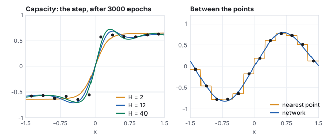
Left: a step target with twelve points, fitted by perceptrons with 2, 12 and 40 hidden units; all fit, the larger ones overshoot slightly at the step. Right: the wave points with a staircase (nearest training point) and the smooth network curve through the same points.
Left: the step target after 3000 epochs with \(H = 2\), 12 and 40 (loss 0.016, 0.010, 0.005). Two units suffice for one step; more units fit the noise around it too. Right: the same twelve wave points answered two ways. The staircase returns the nearest stored example, which is what a table does; the network passes through the same points and is smooth in between.

5.1 Overfitting, and the held-out set

Capacity cuts both ways. A network large enough to trace any curve can trace the noise in its examples as well as the signal, and a training loss that keeps falling then says nothing about how the network will do on data it has not seen. The only honest measure is a held-out set: examples the optimizer never touches, evaluated as training proceeds.
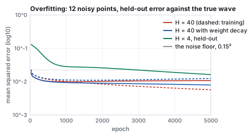
Training and held-out mean squared error against epoch for three fits of twelve noisy wave points: H = 40 whose training error keeps falling while its held-out error bottoms out near epoch 950 and rises; H = 40 with weight decay whose two curves stay together; and H = 4 whose held-out error is higher throughout.
The wave sampled at 12 points with noise of standard deviation 0.15, and the held-out error measured against the true wave on 150 points. Dashed is training error, solid held-out.
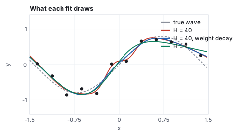
The twelve noisy points with the true wave dashed and three fitted curves: H = 40 wiggling through the noisy points, H = 40 with weight decay smoother, H = 4 smoother still and missing the peaks.
What each fit draws after 5000 epochs. The unregularized \(H = 40\) network bends toward individual noisy points; weight decay keeps it near the true curve.
Worked example (reading the curves) The noise has variance \(0.15^2 = 0.0225\), so a curve that fits the true wave exactly would still have a training error of about 0.0225. After 5000 epochs the \(H = 40\) network has training error 0.0057, a quarter of the noise floor: it has memorized a quarter of the noise. Its held-out error against the true wave reached its minimum, 0.0099, at epoch 950, and rose to 0.0108 by the end; every epoch after 950 made the network worse at the thing it was for. With weight decay \(\lambda = 0.002\) (each step also shrinks every weight by \(\eta\lambda\theta\), penalizing large weights, which are what a sharp wiggle needs) the training error stays at 0.0124 and the held-out error ends at 0.0080, the best of the three. The \(H = 4\) network cannot wiggle at all and ends at 0.0164 held-out: too little capacity is also a failure, just a different one. The recipe that follows from this is the recipe every model in the later chapters uses: a large network, regularized, trained with a held-out set watched and stopped or selected at the held-out minimum.

Other regularizers do the same job by other means: dropout zeroes a random subset of activations at each training step so that no unit can rely on a specific partner; data augmentation (flipping, cropping, recoloring the examples) enlarges the training set with transformations the network should be invariant to; and more data is the regularizer that beats all of them, which is why the diffusion chapter’s largest models are trained on billions of images.

6 · Two more layers: convolution and attention

A fully connected layer on a \(512\times512\) image would have \(786{,}432\) inputs per unit and learn nothing about the fact that a cat in the corner is the same cat as one in the middle. Two layer types encode such structure, and between them they cover every model in the later chapters.

6.1 Convolution

Definition (convolutional layer) A convolutional layer slides one small kernel \(K\) (typically \(3\times3\)) over the image and computes at every position the weighted sum of the neighborhood, \(y_{ij} = \sigma\big(b + \sum_{u,v} K_{uv}\,x_{i+u,\,j+v}\big)\), producing a feature map the size of the input. The nine weights are shared by every position, so the layer has ten parameters instead of millions, and a pattern learned in one place is detected everywhere. A layer learns many kernels (32 to 512), each producing one map, and the next layer convolves over all the maps at once.
Worked example (one output of one kernel) Take the handwritten 3 of the image-space chapter and the kernel \(K = \begin{pmatrix} -1 & 0 & 1 \\ -2 & 0 & 2 \\ -1 & 0 & 1 \end{pmatrix}\), which responds to a vertical edge. At pixel \((12, 15)\) (row, column) the \(3\times3\) neighborhood is three identical rows \((0.99, 0.29, 0)\): ink on the left, paper on the right. The sum is \(-1(0.99) + 0(0.29) + 1(0) - 2(0.99) + 0 + 0 - 1(0.99) + 0 + 0 = -3.96\), and after a ReLU the unit is silent, 0. A second kernel with the opposite sign fires 3.96 here. Over the whole digit the map ranges from \(-3.96\) to \(3.78\), and after the ReLU 23 % of the pixels exceed 0.5: the stroke’s right-facing edges. This kernel was written down; a trained layer’s kernels are found by the gradient, and the first layer of every image network ends up with edge detectors like this one at several orientations, because that is what the loss wants.
Three 20 by 20 panels: the handwritten 3; the raw convolution with the vertical-edge kernel, gray where zero, bright on right-facing edges and dark on left-facing ones; and the same after a ReLU, keeping only the bright edges.
The digit, its convolution with the kernel above (mid-gray is zero), and the feature map after a ReLU.

Stacking convolutions with downsampling between them (pooling, or strided convolution) gives each deeper unit a larger receptive field: edges, then corners and textures, then parts, then objects. Running the stack in reverse with upsampling gives a decoder, and a stack with skip connections from each encoder level to the matching decoder level is the U-Net, the denoiser of the first diffusion models (the diffusion chapter). The filters of the image-space chapter are convolutions with kernels chosen by hand; a convolutional layer is the same operation with kernels chosen by the loss.

6.2 Attention

Definition (attention) Given a set of \(n\) vectors \(\mathbf{x}_1 \dots \mathbf{x}_n\) (words of a sentence, patches of an image), attention computes for each one a query \(\mathbf{q}_i = W_q\mathbf{x}_i\), a key \(\mathbf{k}_i = W_k\mathbf{x}_i\) and a value \(\mathbf{v}_i = W_v\mathbf{x}_i\), and replaces each vector by a weighted average of all the values, weighted by how well its query matches each key: \[ \mathbf{y}_i = \sum_j \alpha_{ij}\,\mathbf{v}_j, \qquad \alpha_{ij} = \frac{\exp(\mathbf{q}_i\cdot\mathbf{k}_j/\sqrt d)}{\sum_{j'}\exp(\mathbf{q}_i\cdot\mathbf{k}_{j'}/\sqrt d)}. \] The weights depend on the data, not only on the position, which is what a convolution cannot do; and every vector can look at every other in one layer.
Worked example (three tokens in two dimensions) Tokens \(\mathbf{x}_1 = (1, 0)\), \(\mathbf{x}_2 = (0, 1)\), \(\mathbf{x}_3 = (1, 1)\), with \(W_q = W_k = I\) and \(W_v = \begin{pmatrix} 0.5 & 1 \\ 1 & 0.5 \end{pmatrix}\), so the values are \((0.5, 1)\), \((1, 0.5)\), \((1.5, 1.5)\). For token 3 the scores \(\mathbf{q}_3\cdot\mathbf{k}_j/\sqrt2\) are \((0.707, 0.707, 1.414)\); the softmax gives \(\alpha_3 = (0.248, 0.248, 0.503)\), and \(\mathbf{y}_3 = 0.248(0.5, 1) + 0.248(1, 0.5) + 0.503(1.5, 1.5) = (1.128, 1.128)\). For token 1 the scores are \((0.707, 0, 0.707)\), the weights \((0.401, 0.198, 0.401)\): token 1 attends to itself and to token 3, which shares its first coordinate, and mostly ignores token 2, which shares nothing. The output \(\mathbf{y}_1 = (1.000, 1.102)\) has mixed in token 3’s value. Change the tokens and the weights change with them.

A transformer is attention layers alternating with small fully connected layers, applied to a sequence of tokens with a positional encoding added so that order is not lost (the same sines and cosines as the NeRF encoding). It is the architecture of CLIP’s text encoder (Section 8), of the language models, and since 2023 of the largest diffusion models, which cut the image into patches and treat them as tokens. The cross-attention by which a caption steers an image model is the same formula with the queries from the image tokens and the keys and values from the caption’s.

7 · Embeddings

Definition (embedding) An embedding of a set of things (words, digits, images) is a map from each thing to a vector in \(\mathbb{R}^d\), learned so that things which behave alike land near each other. Similarity is measured by distance or, more often, by the cosine of the angle between vectors, \[ \cos(\mathbf{u}, \mathbf{v}) = \frac{\mathbf{u}\cdot \mathbf{v}}{\|\mathbf{u}\|\,\|\mathbf{v}\|} \in [-1, 1]. \]
Worked example (cosine similarity) Let \(\mathbf{u} = (3, 4, 0)\), \(\mathbf{v} = (4, 3, 0)\) and \(\mathbf{w} = (-4, 3, 0)\). All three have length 5. \(\mathbf{u}\cdot\mathbf{v} = 12 + 12 + 0 = 24\), so \(\cos(\mathbf{u},\mathbf{v}) = 24/25 = 0.96\): nearly the same direction. \(\mathbf{u}\cdot\mathbf{w} = -12 + 12 + 0 = 0\), so \(\cos(\mathbf{u},\mathbf{w}) = 0\): unrelated. Cosine ignores length, which is why embeddings are usually normalized and only their direction carries meaning.

Nobody places the points. A network puts them where its task goes better; the famous 2013 result was that word vectors trained only to predict neighboring words end up supporting arithmetic, with “king” minus “man” plus “woman” landing near “queen” (Mikolov et al.). The lecture’s embedding exhibit is a smaller and more honest version that you can check to the last digit: the digit-drawing network of the diffusion chapter carries a table of eleven 64-dimensional class vectors (one per digit, one for “no class”) that it learned only from denoising. Nobody told it that a 4 looks like a 9.
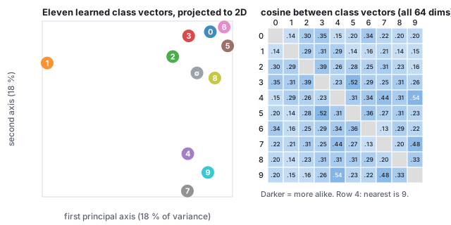
Left: eleven labeled dots, the class embeddings of the trained digit denoiser projected onto their two principal axes; 4 and 9 sit together, 3 and 5 close, 7 near 9, 1 far from everything. Right: a 10 by 10 matrix of cosine similarities between the ten digit vectors, darker where larger.
Read straight from the weight file. Left: the eleven vectors projected onto their two principal axes (18 % and 18 % of the variance; the picture is a shadow of a 64-dimensional arrangement). Right: every pairwise cosine, computed in all 64 dimensions. The nearest neighbor of 4 is 9 (0.54), of 3 is 5 (0.52), of 7 is 9 (0.48), of 2 is 3 (0.39); the 1, which shares strokes with nothing, is far from everything. The network placed digits that share strokes together because a denoiser that knows “this is a 4” and “this is a 9” must do nearly the same work for both.
Worked example (arithmetic on the course’s embeddings, and what it does not do) Word vectors support \(\mathbf{e}_{\text{king}} - \mathbf{e}_{\text{man}} + \mathbf{e}_{\text{woman}}\). Try the same on the digit vectors. \(\mathbf{e}_4 - \mathbf{e}_9 + \mathbf{e}_7\) has, among the classes other than the three operands, the nearest neighbor 2 at cosine 0.31; among all classes, 7 at 0.75. \(\mathbf{e}_3 - \mathbf{e}_5 + \mathbf{e}_8\) lands nearest 9 (0.24) excluding the operands, 8 (0.68) including them. In every case the result stays close to the last operand and no excluded class is near: the digit space has no “subtract a loop, add a stroke” direction, because nothing in the denoising task required one, and eleven points in 64 dimensions are too few to define directions. The word result works because a vocabulary of a hundred thousand words trained on billions of contexts has thousands of relations each realized many times. Embedding arithmetic is a property of a trained space, not of embeddings as such.
Worked example (the eleventh vector) The “no class” vector, which the denoiser reads when it is trained unconditionally (guidance), has length 2.19 against 3.85 to 5.15 for the ten digits, and its cosine with them ranges from 0.19 (to the 1) to 0.47 (to the 5). It sits near the middle of the cloud, shorter than any class vector: the network learned to read “no information” as a small vector in the average direction, which is what a mean is.
See it live Embeddings, read from the weights: the same class table, projected live, with the readout’s cosines using all 64 dimensions.
Hands-on Everything in this chapter’s figures came from two small library files. Run these from the css551/ directory with node -e "…".
  1. Train the perceptron of Section 2 and evaluate it at a point that is not a training point:
    import('./lib/core/mlp-fit.js').then(m=>{const r=m.fit({target:'wave',hidden:12,epochs:3000});
      console.log('loss',r.loss.toFixed(5),'f(0.25)=',m.predict(r.model,0.25).toFixed(4),
      'target',m.TARGETS.wave(0.25).toFixed(4));});
    Expected: loss 0.00079 f(0.25)= 0.4096 target 0.4181. The point \(x = 0.25\) lies between two training points; the network is within 0.01 of the hidden curve there. Change hidden to 2 and the loss stays above 0.05.
  2. Read two class vectors from the trained denoiser and compare them:
    import('./lib/core/pca2.js').then(({cosine})=>{const fs=require('fs');
      const w=new Float32Array(fs.readFileSync('lib/assets/mnist/mlp-denoiser.bin').buffer.slice(0));
      const e=(c)=>Array.from(w.subarray(c*64,(c+1)*64));
      console.log('cos(4,9)=',cosine(e(4),e(9)).toFixed(3),'cos(1,0)=',cosine(e(1),e(0)).toFixed(3));});
    Expected: cos(4,9)= 0.537 cos(1,0)= 0.141, the two extremes of the matrix above. The class table is the first \(11\times64\) floats of the weight file.
  3. In the learning demo, set 40 hidden units and the step target and watch the ramp: it is the \(H = 40\) curve of Section 5, and it overshoots at the step for the same reason.

8 · Encoders, decoders, and one shared space

An encoder is a network that maps a thing to its embedding, \(E : \text{thing} \to \mathbb{R}^d\); a decoder maps back, \(D : \mathbb{R}^d \to \text{thing}\). Trained together to reproduce their input through a narrow middle, \(\min_{E,D} \sum_i \|D(E(x_i)) - x_i\|^2\), they form an autoencoder, and the middle is forced to keep only what matters (Hinton & Salakhutdinov 2006). Stable Diffusion’s autoencoder is exactly this, with a variational twist that keeps the latent well behaved (the diffusion chapter says which): a \(512\times512\times3\) image becomes a \(64\times64\times4\) latent, 48 times fewer numbers.
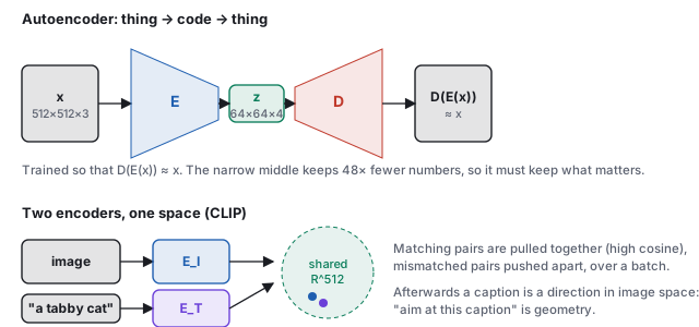
Top: an autoencoder drawn as an input image, an encoder trapezoid narrowing to a small code z, a decoder trapezoid widening back to a reconstruction. Bottom: an image encoder and a text encoder feeding two points into one shared circle labeled R to the 512.
Top: the autoencoder. Only the code \(\mathbf{z}\) crosses the middle, so whatever the decoder needs to rebuild the picture must fit in it; edges, colors and layout survive, sensor noise does not. Bottom: two encoders trained into one space. After training, the arrow from a caption and the arrow from a matching photograph point the same way.

Two encoders, one space. Train an image encoder \(E_I\) and a text encoder \(E_T\) side by side on hundreds of millions of (image, caption) pairs with a contrastive objective: for each batch, a matching pair must have a higher cosine than every mismatched pair,

\[ \mathcal{L} \;=\; -\sum_{i} \log \frac{\exp\big(\cos(E_I(x_i), E_T(t_i))/\tau\big)} {\sum_{j} \exp\big(\cos(E_I(x_i), E_T(t_j))/\tau\big)} , \]

with a temperature \(\tau\). After training, a sentence and a photograph are vectors in the same space, so “aim the picture at this caption” becomes geometry. This is CLIP (Radford et al. 2021), and every concept you can say in words is now a coordinate.
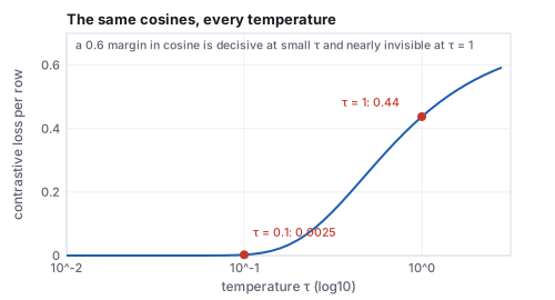
Worked example (the contrastive loss on a batch of two) Two images and their two captions give a \(2\times2\) matrix of cosines \(S_{ij} = \cos(E_I(x_i), E_T(t_j))\); suppose the encoders currently produce \[ S = \begin{pmatrix} 0.8 & 0.2 \\ 0.1 & 0.7 \end{pmatrix}, \] matches on the diagonal. With \(\tau = 0.1\), row 1 becomes \(\exp(8) = 2981.0\) against \(\exp(2) = 7.39\), so the probability assigned to the right caption is \(2981.0/2988.3 = 0.9975\) and the loss for that row is \(-\log 0.9975 = 0.0025\); row 2 gives the same. The batch loss is \(0.005\): these encoders have already learned this batch. Repeat with \(\tau = 1\): the same cosines give probabilities \(0.646\) and a loss of \(0.44\) per row. The temperature is what turns a small cosine margin into a decisive one; CLIP learns \(\tau\) and ends near 0.01, which is why its similarities behave like sharp decisions. The gradient of the loss pushes \(S_{11}\) and \(S_{22}\) up and the off-diagonal entries down, and the only way to move a cosine is to move the vectors: that is how the two encoders come to agree.
The contrastive loss per row for the same two-by-two cosine matrix against temperature on a log axis from 0.01 to 3: zero below 0.05, 0.0025 at 0.1, rising through 0.26 at 0.5 and 0.44 at 1 to 0.6 at 3.
The same cosines at every temperature. Below \(\tau = 0.05\) the loss underflows to zero and the batch teaches nothing more; above 0.5 a margin of 0.6 in cosine is barely a preference. The learned \(\tau\) settles where the batch’s margins are just decisive.

Two consequences of the shared space matter for graphics. A CLIP embedding of a caption is the condition every text-to-image model reads, and its cosine to the embedding of a rendered image is a score that can be optimized: that is the signal DreamFusion follows, through a differentiable renderer, to shape a 3D scene from a sentence. And an embedding is many-to-one, which is the subject of the image-space chapter’s last section.

9 · Coordinate networks

Every network so far was trained on many examples to answer for new ones. A coordinate network is trained on one signal to reproduce that signal: its input is a position, its output the value there. It isolates the function-approximation nature of a network with nothing else in the way, and it is the building block of the radiance fields of the learned-scenes chapter.
Definition (coordinate network) An image of \(N \times N\) pixels is read as a function \(f : [-1, 1]^2 \to [0, 1]^3\), \((x, y) \mapsto (r, g, b)\), sampled at the pixel centres \(x = 2(i + \tfrac12)/N - 1\), \(y = 2(j + \tfrac12)/N - 1\). A coordinate network is a multilayer perceptron (MLP) \(f_\theta\) fitted to those samples by minimizing \(\mathcal{L}(\theta) = \frac{1}{3B}\sum_{i \in \text{batch}} \|f_\theta(x_i, y_i) - c_i\|^2\) over random mini-batches of \(B\) pixels. The fit is scored by the peak signal-to-noise ratio, \(\text{PSNR} = 10\log_{10}(1/\text{MSE})\) for colours in \([0, 1]\).
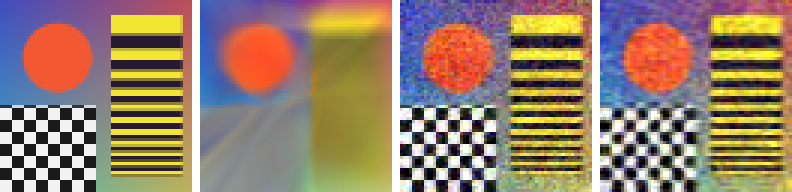
Worked example (one picture, one network) The course’s test card is \(64 \times 64\) pixels: a smooth backdrop, an orange disc, a checkerboard of 4-pixel squares and stripes whose period falls from 16 to 3 pixels. Pixel \((10, 20)\) sits at \((x, y) = (-0.6719, -0.3594)\) and has colour \((0.95, 0.35, 0.20)\). The network has two hidden layers of 48 rectified linear units (ReLU): \(2\cdot48 + 48 = 144\), \(48\cdot48 + 48 = 2352\) and \(48\cdot3 + 3 = 147\) weights, 2,643 in all, against \(64\cdot64\cdot3 = 12{,}288\) numbers in the picture, 4.6 times fewer. There is no held-out image: the training set is the signal, and overfitting is the goal. Trained with Adam (\(\eta = 0.005\), \(B = 256\)), it reaches 11.82 dB after 2,000 steps (MSE 0.0658) and 12.10 dB after 4,000. Split by region at step 2,000: backdrop 23.54 dB, a ring along the disc’s edge 18.72 dB, stripes 11.29 dB, checkerboard 7.56 dB. A learning rate of 0.001 or 0.02 gives 11.63 or 11.99 dB: the blur is not a tuning problem.
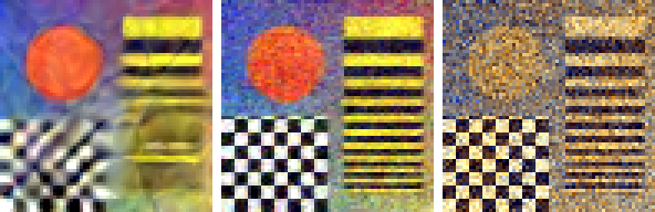
Four 64 by 64 panels: the test card; the plain ReLU fit, a blur with a soft disc and no checkerboard; the Fourier-feature fit, sharp with slight speckle; the SIREN fit, sharp with a softer checkerboard.
The test card and three networks after 2,000 steps of Adam on mini-batches of 256 pixels, computed by lectures/L14-neural-nets-embeddings/analysis/coord-net-figures.mjs with lib/core/coord-net.js: ReLU on raw \((x, y)\), 11.82 dB; ReLU on Fourier features with \(\sigma = 6\), 21.21 dB; SIREN with \(\omega_0 = 30\), 18.89 dB.

9.1 Spectral bias

A network trained by gradient descent fits the low frequencies of its target first and the high frequencies late or never (Rahaman et al. 2019). A ReLU network is continuous and piecewise linear in its input, so a 4-pixel checkerboard asks for a fold every 4 pixels in both directions; in the neural tangent kernel analysis of Tancik et al. (2020) the error’s frequency components shrink at rates that fall with frequency. The same bias is what made the networks of Section 5 smooth between their examples. On a picture with only low frequencies (three soft Gaussian blobs) the plain network reaches 41.54 dB in 2,000 steps: the problem is the signal’s frequency content, not ReLU as such.

9.2 Fourier features and positional encoding

Definition (Fourier features, positional encoding) A Fourier feature mapping replaces the coordinates \(\mathbf v \in [0, 1]^2\) by \(\gamma(\mathbf v) = (\cos 2\pi B\mathbf v, \sin 2\pi B\mathbf v)\), where \(B\) is an \(m \times 2\) matrix with entries drawn once from \(N(0, \sigma^2)\) and never trained; each row is a plane wave with \(|\mathbf b|\) cycles per image width. A positional encoding uses fixed octaves instead, \(\gamma(p) = (\sin 2^k\pi p, \cos 2^k\pi p)_{k = 0}^{L-1}\) for each coordinate, as in NeRF (Mildenhall et al. 2020; \(L = 10\) for position, 4 for direction), and the same construction as the transformer’s positional encoding of Section 6.2 and the diffusion denoiser’s time code.
Worked example (one pixel through the encodings) Pixel \((10, 20)\) has \(\mathbf v = (0.1641, 0.3203)\). With \(\sigma = 6\) the first row of \(B\) is \((-6.6166, -2.0136)\): \(2\pi\,\mathbf b\cdot\mathbf v = -10.8731\), giving the pair \((\cos, \sin) = (-0.1222, 0.9925)\); the second row \((-2.6317, -3.6818)\) gives phase \(-10.1228\) and \((-0.7661, 0.6427)\). Sixteen rows make 32 inputs, so the first layer becomes \(32\cdot48 + 48\) and the network 4,083 weights. The positional encoding of \(x = -0.6719\) with \(L = 6\) has sines \((-0.8577, 0.8819, -0.8315, 0.9239, -0.7071, 1.0000)\) at \(\pi, 2\pi, \ldots, 32\pi\); the \(32\pi\) pair repeats every 2 pixels of a 64-pixel image, the finest pattern that grid holds. Trained like the plain network, the Fourier-feature network reaches 19.24 dB at step 1,000 and 21.21 dB at step 2,000, 9.4 dB above the plain network (8.7 times less error); the stripes rise from 11.29 to 22.30 dB and the checkerboard from 7.56 to 18.74 dB.
Pitfall The scale \(\sigma\) trades blur against noise, and the training pixels hide the noise. Evaluate the network at the corner shared by four pixels and compare with their average, points training never saw. After 2,000 steps:
\(\sigma\)136122448
PSNR on the pixels14.7920.0421.2118.7215.5515.11
PSNR between the pixels18.0622.5821.0316.349.129.02
At \(\sigma = 24\) many waves are faster than the grid’s 32 cycles per width: the fit passes near the pixels and is speckle between them, 6.4 dB worse than on them. A coordinate network is queried between samples whenever the signal is zoomed, resampled or rendered from a new view, so it must be checked off its training grid.
Three Fourier-feature fits: sigma 1 is blurred with smeared stripes; sigma 6 is sharp; sigma 48 is covered in speckle.
Fourier features at \(\sigma = 1, 6, 48\) after 2,000 steps (14.79, 21.21, 15.11 dB on the pixels), same generator and settings as the figure above.

9.3 SIREN: periodic activations

Definition (SIREN) A sinusoidal representation network (Sitzmann et al. 2020) uses \(\mathbf h_{k} = \sin(\omega_0(W_k\mathbf h_{k-1} + \mathbf b_k))\) in every hidden layer, with \(\omega_0 = 30\), and a linear output. Its initialization is part of the method: the first layer draws \(W \sim U(-1/n, 1/n)\), later layers \(W \sim U(-\sqrt{6/n}/\omega_0, \sqrt{6/n}/\omega_0)\), where \(n\) is the layer’s input width. The derivative of a SIREN is again a SIREN (\(\cos\) is a shifted \(\sin\)), so its gradients and Laplacians are smooth; a ReLU network’s second derivative vanishes almost everywhere. The paper fits images, audio, video, signed distance functions and solutions of the Poisson, Helmholtz and wave equations.
Worked example (the initialization, and what breaks without it) With \(n = 2\) inputs the first layer has \(|W| \le 0.5\); with biases up to \(1/\sqrt2\), the phase \(\omega_0|W\mathbf p + \mathbf b|\) reaches 51 radians, 8 periods across the image. A hidden layer of width 48 has \(|W| \le \sqrt{6/48}/30 = 0.0118\), so \(\omega_0|W| \le 0.354\), and the mean phase \(|\omega_0 z|\) in layer 2 over the image is 2.35 radians. Omitting the \(1/\omega_0\) raises that mean to 23.87 radians: each sine sees a phase spread over many periods, its output is a scramble of its input, and the fit at step 2,000 falls from 18.89 to 13.27 dB. \(\omega_0\) plays the role of \(\sigma\): at \(\omega_0 = 1, 5, 10, 30, 90\) the PSNR on the pixels is 11.05, 11.87, 13.34, 18.89, 17.95 dB and between them 12.86, 14.16, 16.26, 22.56, 17.82 dB. With the same 2,643 weights as the plain network, the SIREN leads early (16.01 dB at step 300 against 14.57 for Fourier features) and ends at 20.16 dB at step 4,000.

9.4 Multiresolution hash encoding

Instant NGP (Müller et al. 2022) trains the encoding itself. At each of \(L\) grid resolutions \(N_l = \lfloor N_{\min} b^l\rfloor\) the point’s cell is found, the feature vectors (\(F\) numbers each) of its corners are read from a table of \(T\) entries and interpolated, and the \(L \cdot F\) results are concatenated and passed to a small MLP. Coarse grids have one entry per vertex; fine grids are hashed, \(h(\mathbf v) = (v_1 \cdot 1 \oplus v_2 \cdot 2654435761) \bmod T\), and colliding vertices share an entry. With \(T = 2^{14}\), the corners of one cell, \((37, 12), (38, 12), (37, 13), (38, 13)\), hash to 13417, 13418, 11736, 11739. With \(L = 16\), \(F = 2\), \(T = 2^{19}\) the tables hold at most \(16\cdot2^{19}\cdot2 = 16{,}777{,}216\) parameters, yet each point reads only 4 entries per level in 2D, so a training step is cheap; in 2D with \(N_{\min} = 16\), \(N_{\max} = 2048\) (\(b = 1.3819\)) the first 12 levels fit densely and the last 4 are hashed. The paper reports training “in a matter of seconds”. The same recipe, encoding plus MLP plus loss, represents video \((x, y, t)\), shapes as signed distances \((x, y, z)\), and radiance fields \((x, y, z, \text{direction}) \mapsto (\text{density}, \text{colour})\), whose loss compares rendered pixels with photographs (the learned-scenes chapter).

See it live Coordinate networks: the three networks of this section train side by side in the browser, with sliders for \(\sigma\) and \(\omega_0\); training pauses at step 2,000 on the values quoted here.
Hands-on Run from the css551/ directory with node -e "…".
  1. Train the three networks of this section for 1,000 steps:
    import('./lib/core/coord-net.js').then(C=>{const img=C.makeImage('card');
      for(const k of ['relu','fourier','siren']){const t=C.makeTrainer(k,img);
        for(let s=0;s<1000;s++)t.step();
        console.log(k,C.paramCount(t.net),C.psnr(C.mse(C.render(t.net),img)).toFixed(2));}});
    Expected: relu 2643 11.67, fourier 4083 19.24, siren 2643 18.14.
  2. Encode pixel \((10, 20)\) with the Fourier features:
    import('./lib/core/coord-net.js').then(C=>{const net=C.makeNet('fourier',{sigma:6});
      const o=new Float64Array(32);C.encode(net,-0.671875,-0.359375,o);
      console.log(o[0].toFixed(4),o[16].toFixed(4),o[1].toFixed(4),o[17].toFixed(4));});
    Expected: -0.1222 0.9925 -0.7661 0.6427, the two \((\cos, \sin)\) pairs of the worked example.
  3. In the demo, play to step 2,000, then set \(\sigma = 48\) and play again: the Fourier panel turns to speckle. Switch the picture to blobs and compare the plain network’s PSNR with its test-card value.

10 · The papers

YearPaperWhat it added
1986Rumelhart, Hinton & Williamsbackpropagation
1989 / 1991Cybenko; Hornikuniversal approximation
1998LeCun, Bottou, Bengio & Haffnerconvolutional networks trained end to end (on the digits of this text)
2006Hinton & Salakhutdinovdeep autoencoders
2013Mikolov et al., word2vecembeddings that support arithmetic
2015Kingma & Ba, Adamthe default optimizer
2016He et al., ResNetskip connections; depth without vanishing gradients
2017Vaswani et al., Transformerattention as the whole architecture
2020Ho, Jain & Abbeel, DDPMpredict the noise; it works at scale
2021Radford et al., CLIPtext and images, one space
2019Rahaman et al.spectral bias: networks learn low frequencies first
2020Mildenhall et al., NeRFpositional encoding of coordinates; radiance fields
2020Tancik et al.Fourier features; the scale as a bandwidth
2020Sitzmann et al., SIRENsine activations and their initialization
2022Müller et al., Instant NGPmultiresolution hash encoding

11 · Exercises

Exercise 1 (forward pass) With the original weights of Section 1, evaluate \(f(-0.4)\).
Solution \(z = (-0.4 + 0.5,\; 0.4 + 0.5) = (0.1, 0.9)\), \(a = (0.0997, 0.7163)\), \(f = 0.1 + 0.8\times0.0997 - 0.6\times0.7163 = 0.1 + 0.0798 - 0.4298 = -0.2500\). The two units have swapped roles: the network is not symmetric in \(x\) because \(w^{(2)}\) is not.
Exercise 2 (one more step) Starting from the updated weights of Section 2, compute the gradient with respect to \(b_2\) only and take a second step. Does the loss keep falling?
Solution After the first step \(f = 0.4814\), so \(\delta = 2(0.4814 - 0.3) = 0.3628\) and \(\partial\mathcal{L}/\partial b_2 = 0.3628\). Moving only \(b_2\): \(b_2 = 0.0374 - 0.0363 = 0.0011\), \(f = 0.4451\), loss \(0.0211\), down from \(0.0329\). The full step (all seven weights) would fall faster, but every single weight’s step is in a descending direction on its own; that is what a gradient is.
Exercise 3 (activations) Replace \(\tanh\) by ReLU in the forward pass of Section 1 (same weights, \(x = 0.4\)). What is \(f\), and what is \(\partial\mathcal{L}/\partial w^{(1)}_2\) for the target \(y = 0.3\)?
Solution \(z = (0.9, 0.1)\), both positive, so \(a = z = (0.9, 0.1)\) and \(f = 0.1 + 0.72 - 0.06 = 0.76\). \(\delta = 0.92\); the ReLU derivative is 1 for both units, so \(\partial/\partial w^{(1)}_2 = \delta\, w^{(2)}_2 \cdot 1 \cdot x = 0.92\times(-0.6)\times0.4 = -0.221\), against \(-0.149\) with \(\tanh\), whose derivative 0.99 at \(z_2 = 0.1\) barely damped it and whose derivative 0.49 at \(z_1 = 0.9\) halved the other unit’s gradient. Had \(z_2\) been negative, the ReLU gradient through it would be exactly zero: a dead unit.
Exercise 4 (two layers, one weight) In the network of Section 3, by how much would the loss change if only \(W^{(2)}_{11}\) moved by \(-0.01\)? Estimate from its gradient and compare with a recomputed forward pass.
Solution Gradient \(0.0341\), so the predicted change is \(-0.01\times0.0341 = -0.00034\), from 0.00119 to 0.00085. Recomputing: \(z^{(2)}_1 = 0.59(0.7163) - 0.4(0.0997) = 0.3827\), \(a = 0.3650\), \(f = 0.1 + 0.2920 - 0.0625 = 0.3295\), loss \(0.00087\). The linear estimate is good to two digits at this step size, which is the assumption gradient descent rests on.
Exercise 5 (Adam’s second step) Suppose the gradient at step 2 is the same as at step 1 for one weight, \(g = 0.6265\). Compute the Adam update at \(t = 2\) with \(\eta = 0.01\).
Solution \(m_2 = 0.9(0.0627) + 0.1(0.6265) = 0.1190\), \(\hat m = 0.1190/(1 - 0.81) = 0.6265\); \(v_2 = 0.999(0.000392) + 0.001(0.3925) = 0.000784\), \(\hat v = 0.000784/(1 - 0.998) = 0.3925\); update \(= 0.01\times0.6265/0.6265 = 0.01\). A consistent gradient keeps the step at exactly \(\eta\); the bias correction is what makes the early steps come out this cleanly.
Exercise 6 (capacity) The perceptron with \(H\) units has \(3H + 1\) weights. How many units would it take to store twelve arbitrary points exactly, and why does the \(H = 12\) fit in Section 2 nevertheless stop at loss \(8\times10^{-4}\) rather than 0?
Solution Twelve points are 12 constraints; \(H = 4\) already has 13 weights, so in principle enough freedom exists. Freedom is not reachability: gradient descent finds a nearby smooth solution, the target points carry noise (\(\pm0.03\)), and a smooth curve does not pass through noisy points exactly. The residual is the noise, not a shortage of weights; the \(H = 40\) run stops at a similar loss.
Exercise 7 (overfitting, with the library) Using lib/core/mlp-fit.js, train \(H = 40\) on makeSamples('wave', 12, 3, 0.15) for 5000 epochs and measure the mean squared error against TARGETS.wave on 150 evenly spaced points every 250 epochs. Where is the minimum?
Solution The generator’s run finds the held-out minimum near epoch 950 (0.0099) with the error rising to 0.0108 by 5000; a run with the library’s trainStep and the same seed reproduces the curve to the precision of the figure. A different seed moves the minimum by a few hundred epochs but not its existence: with 12 noisy points and 121 weights, late training always fits noise.
Exercise 8 (convolution) Apply the kernel of Section 6 to a neighborhood whose rows are \((0, 0.29, 0.99)\), the mirror image of the worked one. Then apply the transposed kernel (the horizontal-edge detector) to the original neighborhood.
Solution Mirror: \(+3.96\), a right-facing edge, and the ReLU passes it. Transposed kernel on the original: the rows are identical, so the top row contributes \(-(0.99 + 2\cdot0.29 + 0)\) and the bottom row \(+(0.99 + 2\cdot0.29 + 0)\): exactly 0. A horizontal-edge detector sees nothing in a vertical edge; the two kernels are orthogonal detectors, and a trained first layer contains both.
Exercise 9 (attention) In the three-token example, what is \(\mathbf{y}_2\)? Then double all three tokens and say what changes in the weights.
Solution By symmetry with token 1, scores \((0, 0.707, 0.707)\), weights \((0.198, 0.401, 0.401)\), \(\mathbf{y}_2 = (1.102, 1.000)\). Doubling the tokens quadruples every dot product (both query and key double), so the scores become \((0, 2.83, 2.83)\) and the weights sharpen to \((0.029, 0.486, 0.486)\): attention’s temperature is the scale of the vectors, which is why the \(\sqrt d\) is there and why the inputs are normalized before each layer.
Exercise 10 (embeddings) From the cosine matrix in Section 7, which digit is farthest from all others, and what feature of its shape explains it?
Solution The 1: its nearest neighbor (3) has cosine only 0.31, the lowest nearest-neighbor value of any class. A 1 is a single stroke and shares no loop or crossbar with anything; a denoiser that has decided the image is a 1 does different work than for any other class, so the class vector ended up alone.
Exercise 11 (memorizing one signal) A coordinate network with two hidden layers of width \(H\), two inputs and three outputs is fitted to a \(64\times64\) colour image. For which \(H\) does it have as many weights as the image has numbers? Why does a network with fewer weights still reach 21 dB on the test card once it has Fourier features?
Solution Weights \(= 2H + H + H^2 + H + 3H + 3 = H^2 + 7H + 3\); setting this to 12,288 gives \(H \approx 107.5\), so \(H = 108\) (12,423 weights). At \(H = 48\) the network has 2,643 weights (4,083 with 16 Fourier frequencies), so it cannot store the pixels one by one: it compresses them into a function. The test card is mostly smooth regions and periodic patterns, which a sum of waves describes with few numbers; the residual error (21.21 dB, MSE 0.0076) is what that compression loses.
Exercise 12 (the scale, with the library or the demo) Using lib/core/coord-net.js (or the demo’s \(\sigma\) slider and its pause at step 2,000), train the Fourier-feature network at \(\sigma = 3\) and \(\sigma = 24\), and evaluate each at the corners shared by four pixels against the four pixels’ mean. Which \(\sigma\) would you choose for a network that will be rendered at twice the resolution, and why does the PSNR on the pixels alone mislead?
Solution The generator gives \(\sigma = 3\): 20.04 dB on the pixels, 22.58 dB between them; \(\sigma = 24\): 15.55 and 9.12 dB. Rendering at twice the resolution evaluates three new points for every training pixel, all between samples, so \(\sigma = 3\) (or 6, 21.03 dB between) is the choice. The training PSNR at \(\sigma = 24\) is only 4.5 dB below \(\sigma = 3\), while between the pixels the gap is 13.5 dB: high frequencies the grid cannot represent fit the samples and fill the gaps with noise.