This chapter links to the course’s interactive demos and to original papers on the open web, and it uses MathJax for its formulas. Read it through the course website (or download the file and open it in a browser); a Canvas inline preview will reach neither the demos nor the math. All chapters.

Diffusion Models

Diffusion models began in a 2015 paper by Sohl-Dickstein and colleagues that borrowed its idea from non-equilibrium thermodynamics. Sohl-Dickstein et al., arXiv:1503.03585

A diffusion model answers the one-to-many problem of the space of images with noise: walk real images into noise on a schedule you control, train a network to undo one small step, then start from fresh noise and undo all the way. This chapter writes the recipe out, derives the exact denoiser that the course’s demos compute, shows that predicting the image, the noise, the score and the velocity are one function in four coordinates, says where the training loss comes from, states the samplers and measures how their accuracy depends on the number of steps, presents flow matching as the straight-line version of the same idea, explains guidance and its cost, follows the three scalings that turn a digit-drawing network into Stable Diffusion, and asks how any of it is evaluated. Every stage is shown twice: on a dataset of dots small enough to draw the whole thing, and on real digits, including samples drawn from the course’s own trained network. It closes with what still breaks and the papers.

Contents
  1. The forward process, and the schedule
  2. The exact denoiser, in four parameterizations
  3. Training, and where the loss comes from
  4. Sampling: steps, stochasticity, and the ODE underneath
  5. Flow matching: the straight-line version
  6. From lookup table to network
  7. Guidance
  8. From digits to Stable Diffusion: the three scalings
  9. Evaluation: how a generator is judged
  10. What still breaks, and what graphics keeps
  11. The papers
  12. Exercises

1 · The forward process, and the schedule

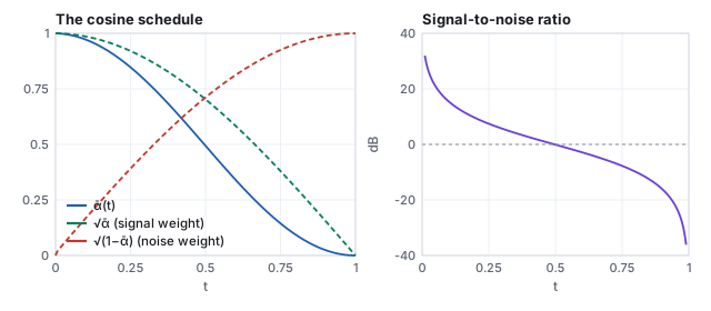
Fix a schedule \(\bar\alpha(t)\) that falls from \(1\) at \(t=0\) to \(0\) at \(t=1\) (the course’s demos and this chapter use the cosine schedule of Nichol & Dhariwal 2021). The forward process mixes a clean image with Gaussian noise in a proportion set by \(t\):
Definition (forward process) \[ \mathbf{x}_t \;=\; \sqrt{\bar\alpha(t)}\;\mathbf{x}_0 \;+\; \sqrt{1-\bar\alpha(t)}\;\boldsymbol{\epsilon}, \qquad \boldsymbol{\epsilon}\sim\mathcal{N}(0, I). \] The two weights are chosen so that \(\bar\alpha + (1 - \bar\alpha) = 1\): if \(\mathbf{x}_0\) has unit variance, so does every \(\mathbf{x}_t\). The signal-to-noise ratio is \(\bar\alpha/(1-\bar\alpha)\).
Left: the cosine schedule alpha-bar falling from 1 to 0 over t in [0,1], with the signal weight root alpha-bar and the noise weight root one minus alpha-bar. Right: the signal-to-noise ratio in decibels, crossing zero at t = 0.5.
The cosine schedule. \(\bar\alpha\) is the fraction of the variance that is still signal; the two square roots are the weights in the definition. The signal-to-noise ratio crosses 0 dB at \(t = 0.5\), where signal and noise have equal power; it falls about 3 dB per tenth of \(t\) through the middle and steepens toward both ends (6 dB between 0.1 and 0.2, and again between 0.8 and 0.9).
\(t\)\(\bar\alpha\)\(\sqrt{\bar\alpha}\)\(\sqrt{1-\bar\alpha}\)SNR (dB)PSNR of the digit below (dB)
0.10.9720.9860.16715.421.2
0.20.8990.9480.3189.516.4
0.30.7870.8870.4625.712.3
0.40.6480.8050.5942.610.0
0.50.4940.7030.711−0.18.5
0.60.3410.5840.812−2.97.3
0.70.2030.4510.893−5.96.4
0.80.0940.3070.952−9.85.2
0.90.0240.1550.988−16.13.3
1.0001−∞3.3
Eleven images of a handwritten 7 with increasing Gaussian noise, from clean at t = 0 to unrecognizable static at t = 1; the digit is still readable at t = 0.5 and gone by t = 0.8.
One digit walked forward, \(t = 0, 0.1, \dots, 1\), with a fixed noise vector \(\boldsymbol\epsilon\) scaled up as \(t\) grows. The last column of the table is the PSNR between each panel and the clean digit (the image-space chapter defines it). The 7 survives to \(t \approx 0.6\) because its coarse structure (a bar and a stroke) is a large-scale feature, and large-scale features are the last to drown; compare the cosine-basis reconstruction in the image-space chapter, where the same coarse structure was the first to be recovered.

Nothing is learned here. At \(t=1\) every image has become the same standard Gaussian, which is the whole point: that is the one distribution we can sample from trivially.
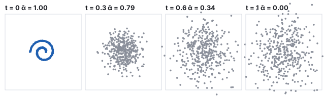
Four panels of 400 points: a tight blue spiral at t = 0, a blurred spiral at t = 0.3, a nearly shapeless cloud at t = 0.6, and an isotropic Gaussian cloud at t = 1.
The same walk on a dataset small enough to draw whole: 400 points on a spiral in \(\mathbb{R}^2\). Each point is an “image” with two pixels. By \(t = 0.6\) the spiral is gone; by \(t = 1\) the cloud is the standard Gaussian, and it would be the same cloud for a ring, two moons, or a million photographs.

1.1 Which schedule

The schedule is a choice, and the first one was different. DDPM defined the process in 1,000 discrete steps with per-step noise variances \(\beta_k\) rising linearly from \(10^{-4}\) to \(0.02\), giving \(\bar\alpha_k = \prod_{j \le k}(1 - \beta_j)\). The cosine schedule was introduced because the linear one destroys the signal too early: half of the steps are spent on images that are already noise.
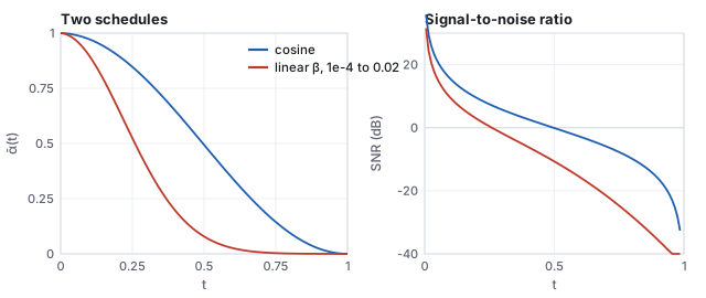
Left: alpha-bar against t for the cosine schedule, a smooth S from 1 to 0, and the linear-beta schedule, which drops much faster and is near zero by t = 0.6. Right: the two signal-to-noise curves in decibels, the linear one about 10 dB below the cosine one through the middle.
The two schedules on the same axes. At \(t = 0.5\) the cosine schedule holds \(\bar\alpha = 0.494\) (0 dB); the linear one holds 0.079 (\(-10.7\) dB). At \(t = 0.7\) the linear schedule is at 0.007, an image that is 99 % noise, with three tenths of the steps still to come.
\(t\)0.10.30.50.70.9
\(\bar\alpha\), cosine0.9720.7870.4940.2030.024
\(\bar\alpha\), linear \(\beta\)0.8970.3960.0790.0070.0003
SNR, cosine (dB)15.45.7−0.1−5.9−16.1
SNR, linear (dB)9.4−1.8−10.7−21.5−35.6

A schedule is only a way of spacing the noise levels the network sees; what matters is that the levels cover the range from “almost clean” to “almost noise” evenly in signal-to-noise ratio, which the cosine schedule does at about 3 dB per tenth. Later work (the EDM formulation of Karras and others, 2022) parametrizes the process directly by the noise standard deviation \(\sigma\) and treats the schedule and the sampler’s step spacing as separate design choices; the demos’ \(t\) is one such parametrization.

See it live A real picture, dissolving: the course’s Cornell render as \(\mathbf{x}_0\) beside \(\mathbf{x}_t\) for the \(t\) on the slider, with \(\bar\alpha\), SNR and PSNR.

2 · The exact denoiser, in four parameterizations

The learned part answers a local question: given \(\mathbf{x}_t\) and \(t\), where was \(\mathbf{x}_0\)? For a finite dataset \(\{\mathbf{x}^{(i)}\}\) the best possible answer is computable in closed form. Since \(\mathbf{x}_t\) given \(\mathbf{x}_0=\mathbf{x}^{(i)}\) is Gaussian with mean \(\sqrt{\bar\alpha}\,\mathbf{x}^{(i)}\) and variance \(1-\bar\alpha\), Bayes’ rule gives the posterior mean

The exact denoiser \[ \hat{\mathbf{x}}_0(\mathbf{x}_t, t) \;=\; \mathbb{E}[\mathbf{x}_0\mid\mathbf{x}_t] \;=\; \sum_i w_i\, \mathbf{x}^{(i)}, \qquad w_i \;\propto\; \exp\!\Big(-\frac{\|\mathbf{x}_t - \sqrt{\bar\alpha}\,\mathbf{x}^{(i)}\|^2}{2(1-\bar\alpha)}\Big), \] a softmax-weighted average of the training points, weighted by how well each explains \(\mathbf{x}_t\). It minimizes the expected squared error among all functions of \(\mathbf{x}_t\).
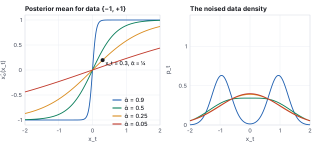
Worked example (two training points, unrolled) Let the dataset be two scalars, \(x^{(1)} = -1\) and \(x^{(2)} = +1\), and take a time where \(\bar\alpha = \tfrac14\), so \(\sqrt{\bar\alpha} = \tfrac12\) and \(1-\bar\alpha = \tfrac34\). Observe \(x_t = 0.3\).
scaled data\(\tfrac12 x^{(1)} = -0.5\),   \(\tfrac12 x^{(2)} = +0.5\)
squared distances\((0.3 + 0.5)^2 = 0.64\),   \((0.3 - 0.5)^2 = 0.04\)
logits \(-d^2/(2\cdot\tfrac34)\)\(-0.4267\),   \(-0.0267\)
softmax weights\(e^{-0.4267} = 0.653\), \(e^{-0.0267} = 0.974\); normalized: \(0.401\), \(0.599\)
posterior mean\(\hat x_0 = 0.401\times(-1) + 0.599\times(+1) = 0.197\)
A pull toward the nearer point, not a jump onto it. The figure draws the whole function \(\hat x_0(x_t)\) for four noise levels.
Left: the posterior mean as a function of x_t for the data set minus one and plus one, at alpha-bar 0.9, 0.5, 0.25 and 0.05: a sharp step near zero noise flattening to a gentle line at high noise, with the worked point marked. Right: the noised data density at the same four levels, two sharp bumps merging into one broad bump.
Left: \(\hat x_0(x_t)\) for data \(\{-1, +1\}\). At \(\bar\alpha = 0.9\) (little noise) it is nearly a step: whichever side of 0 you observe, the answer is that training point. At \(\bar\alpha = 0.05\) (mostly noise) it is nearly flat: the best guess is close to the data mean, 0, wherever you are. The dot is the worked example. Right: the density of \(x_t\) at the same four levels; the denoiser is, up to a factor, the slope of the logarithm of these curves.

Two limits of the figure matter. As \(t\to0\), \(1-\bar\alpha\to0\), the weights become one-hot, and \(\hat x_0\) becomes exactly the nearest training point: the exact denoiser memorizes. As \(t \to 1\) the weights become equal and \(\hat x_0\) becomes the data mean: at high noise the best guess is the average image, which is why the first steps of every sampling run look like a gray blur.

2.1 One function, four coordinates

The same function has four names, and a network may be trained to output any of them.

the network predictsformularecover \(\hat{\mathbf{x}}_0\) byused by
the clean image \(\hat{\mathbf{x}}_0\)the posterior mean aboveitselfthe course’s network
the noise \(\hat{\boldsymbol\epsilon}\)\((\mathbf{x}_t - \sqrt{\bar\alpha}\,\hat{\mathbf{x}}_0)/\sqrt{1-\bar\alpha}\)\((\mathbf{x}_t - \sqrt{1-\bar\alpha}\,\hat{\boldsymbol\epsilon})/\sqrt{\bar\alpha}\)DDPM, Stable Diffusion 1
the score \(\nabla\log p_t\)\((\sqrt{\bar\alpha}\,\hat{\mathbf{x}}_0 - \mathbf{x}_t)/(1-\bar\alpha) = -\hat{\boldsymbol\epsilon}/\sqrt{1-\bar\alpha}\)from \(\hat{\boldsymbol\epsilon}\)score-based models, the SDE view
the velocity \(\hat{\mathbf{v}}\)\(\sqrt{\bar\alpha}\,\hat{\boldsymbol\epsilon} - \sqrt{1-\bar\alpha}\,\hat{\mathbf{x}}_0\)\(\sqrt{\bar\alpha}\,\mathbf{x}_t - \sqrt{1-\bar\alpha}\,\hat{\mathbf{v}}\)Stable Diffusion 2, distillation

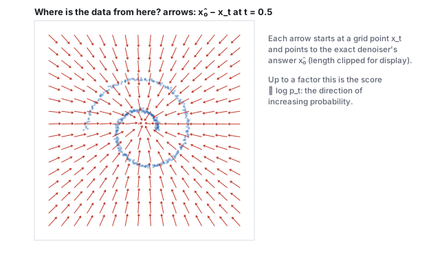
The score identity is Tweedie’s formula: the posterior mean is a step up the gradient of the log density of the noised data, which is the vector field the next figure draws as arrows. Predicting \(\boldsymbol\epsilon\) is ill-conditioned at low noise (the recovery divides by \(\sqrt{\bar\alpha} \approx 1\), fine) and predicting \(\mathbf{x}_0\) is ill-conditioned at high noise (the network must guess an image from static); the velocity \(\mathbf{v}\), an angle between the two, is well-conditioned at both ends, which is why it won out for models that must work with few steps.
Worked example (the four coordinates at one point of the spiral run) At step 15 of the 50-step run of Section 4, \(t = 0.6993\), \(\sqrt{\bar\alpha} = 0.4517\), \(\sqrt{1-\bar\alpha} = 0.8922\), the particle is at \(\mathbf{x}_t = (0.8662, 1.0562)\) and the exact denoiser says \(\hat{\mathbf{x}}_0 = (0.0367, 0.1490)\). Then \(\hat{\boldsymbol\epsilon} = (\mathbf{x}_t - 0.4517\,\hat{\mathbf{x}}_0)/0.8922 = (0.9523, 1.1084)\); the score is \(-\hat{\boldsymbol\epsilon}/0.8922 = (-1.067, -1.242)\), pointing back toward the origin, where the data’s mass is; and \(\hat{\mathbf{v}} = 0.4517\,(0.9523, 1.1084) - 0.8922\,(0.0367, 0.1490) = (0.397, 0.368)\). Recovering the image from the velocity: \(0.4517\,\mathbf{x}_t - 0.8922\,\hat{\mathbf{v}} = (0.3913 - 0.3546,\; 0.4771 - 0.3281) = (0.037, 0.149)\), the same \(\hat{\mathbf{x}}_0\). Four vectors, one fact about where the particle came from.
The spiral drawn faintly with a grid of red arrows over it at t = 0.5; every arrow points from its grid position toward the spiral, converging on the data.
The exact denoiser at \(t = 0.5\) on the spiral, as a field: each arrow runs from a point \(\mathbf{x}_t\) to its estimate \(\hat{\mathbf{x}}_0\) (lengths clipped for legibility). Far from the data every arrow points at the data’s center of mass; near the spiral the arrows resolve its arms. A sampler is a particle that follows this field while the field sharpens.
See it live The mechanism, on dots (400 points on a spiral, the exact denoiser, arrows for the score field, DDIM versus DDPM stepping), then real digits, the exact denoiser (2,000 MNIST digits as points of \(\mathbb{R}^{400}\)).

3 · Training, and where the loss comes from

For a million photographs the sum in the exact denoiser is unaffordable and, worse, useless: it can only return the photographs. So the function is approximated by a network, and the training loop is one line: pick an image \(\mathbf{x}_0\) and a random \(t\), draw \(\boldsymbol\epsilon\), form \(\mathbf{x}_t\), ask the network for the noise (or for the image), and minimize the squared error,

\[ \mathcal{L}(\theta) \;=\; \mathbb{E}_{\mathbf{x}_0,\, t,\, \boldsymbol\epsilon} \Big[\, \big\|\boldsymbol\epsilon - \boldsymbol\epsilon_\theta(\mathbf{x}_t, t)\big\|^2 \Big]. \]
for step in range(N):
    x0  = random_batch(images)            # clean images
    t   = uniform(0, 1, size=batch)       # a noise level per image
    eps = normal(0, 1, shape=x0.shape)    # the noise
    xt  = sqrt(abar(t)) * x0 + sqrt(1 - abar(t)) * eps
    loss = mean((net(xt, t, label) - target)**2)   # target = eps, or x0, or v
    loss.backward(); optimizer.step()

Every step is a small, well-posed regression against a target the trainer generated itself, which is why diffusion trains stably where adversarial models fought their own training. This is DDPM (Ho, Jain & Abbeel 2020); the idea comes from Sohl-Dickstein et al. 2015, who borrowed it from nonequilibrium thermodynamics, and the same function was reached from the score side by Song & Ermon 2019. The course’s own network (the lecture’s last exhibit) is a class-conditional perceptron with three hidden layers of 512 units (SiLU activations, the networks chapter) and 1,002,064 weights, trained by exactly this loop with the Adam optimizer on the 60,000 MNIST training digits for fifteen minutes on a laptop CPU (41,210 steps of batch 512), predicting the clean image (tools/train-mlp.py). Section 6 shows what it draws.

3.1 Where the squared error comes from

The loss is not an arbitrary choice; it is what maximizing the likelihood of the data reduces to. The reverse process is a chain of Gaussians \(p_\theta(\mathbf{x}_{t-1}\mid\mathbf{x}_t)\), and the log probability it assigns to a training image is bounded below by the evidence lower bound, a sum over steps of the divergence between the model’s reverse step and the true one:

The variational bound \[ -\log p_\theta(\mathbf{x}_0) \;\le\; \sum_{t}\; \mathbb{E}\Big[\mathrm{KL}\big(q(\mathbf{x}_{t-1}\mid\mathbf{x}_t, \mathbf{x}_0)\;\|\;p_\theta(\mathbf{x}_{t-1}\mid\mathbf{x}_t)\big)\Big] + \text{const}. \] The true reverse step \(q(\mathbf{x}_{t-1}\mid\mathbf{x}_t, \mathbf{x}_0)\) is Gaussian with a known mean that depends on \(\boldsymbol\epsilon\); the model’s is Gaussian with a mean that depends on \(\boldsymbol\epsilon_\theta\); and the divergence between two Gaussians of equal variance is the squared distance between their means over twice the variance. Each term is therefore \(\lambda_t\,\|\boldsymbol\epsilon - \boldsymbol\epsilon_\theta\|^2\) with a weight \(\lambda_t = \beta_t^2/\big(2\sigma_t^2\alpha_t(1 - \bar\alpha_t)\big)\) that depends on the schedule.

DDPM’s observation was that dropping \(\lambda_t\) (weighting every noise level equally) gives better samples than the exact bound, because the bound over-weights the low-noise steps that barely change an image. The one-line loss above is that “simple” objective. Later work reweights on purpose: weighting by the signal-to-noise ratio, or with the velocity parameterization, which is the simple loss in different coordinates. Whichever weighting is used, the minimizer at each \(t\) is the posterior mean of Section 2: the loss is a way of approximating the exact denoiser, and the weights only say which noise levels get the network’s attention.

3.2 How the condition gets in

mechanismhow the network reads the conditionwhere
embedding added to the time embeddinga learned vector per class, summed into the hidden statethe course network; class-conditional ImageNet models
cross-attentionimage tokens attend to the caption’s token embeddings at every layer (the networks chapter)Stable Diffusion, Imagen
concatenationthe condition is an image (a depth map, a mask, a low-resolution version) stacked onto \(\mathbf{x}_t\) as extra channelssuper-resolution, inpainting, ControlNet’s input
adaptera trained copy of the encoder half reads the condition and adds its features to the frozen modelControlNet
guidancethe difference between conditional and unconditional predictions, amplified at sampling timeSection 7

4 · Sampling: steps, stochasticity, and the ODE underneath

Start from \(\mathbf{x}_T\sim\mathcal{N}(0,I)\) and step \(t\) down a chosen sequence \(t_K > \dots > t_0 = 0\). At each step form \(\hat{\mathbf{x}}_0\) from the denoiser, recover the implied noise \(\hat{\boldsymbol\epsilon}\), and move to the next time. The DDIM family (Song, Meng & Ermon 2021) writes the update as

Definition (one reverse step) \[ \mathbf{x}_{t'} \;=\; \sqrt{\bar\alpha(t')}\;\hat{\mathbf{x}}_0 \;+\; \sqrt{1-\bar\alpha(t') - \sigma^2}\;\hat{\boldsymbol\epsilon} \;+\; \sigma\,\mathbf{z}, \qquad \mathbf{z}\sim\mathcal{N}(0,I), \] with \(\sigma = 0\) giving the deterministic DDIM sampler and \(\sigma\) at its DDPM value giving the original stochastic one.

Read it as: re-noise the current best guess of the clean image to the next, slightly lower, noise level, reusing the noise you believe is already in the picture (\(\sigma = 0\)) or partly replacing it with fresh noise (\(\sigma > 0\)). The forward formula and the reverse step are the same equation; the only new ingredient is that \(\mathbf{x}_0\) is unknown and \(\hat{\mathbf{x}}_0\) stands in for it.

Worked example (one DDIM step, from the spiral run) Fifty steps from \(t = 0.999\) to \(0\). Take the first particle of the run at step 15, where \(t = 0.6993\) and the next time is \(t' = 0.6793\).
schedule\(\bar\alpha(t) = 0.2040\), \(\sqrt{\bar\alpha} = 0.4517\), \(\sqrt{1-\bar\alpha} = 0.8922\);   \(\bar\alpha(t') = 0.2297\), \(\sqrt{\bar\alpha'} = 0.4792\), \(\sqrt{1-\bar\alpha'} = 0.8777\)
where the particle is\(\mathbf{x}_t = (0.8662,\; 1.0562)\)
exact denoiser\(\hat{\mathbf{x}}_0 = (0.0367,\; 0.1490)\): still near the data’s center, since most of the picture is noise
implied noise\(\hat{\boldsymbol\epsilon} = (\mathbf{x}_t - 0.4517\,\hat{\mathbf{x}}_0)/0.8922 = (0.9523,\; 1.1084)\)
next position (\(\sigma = 0\))\(\mathbf{x}_{t'} = 0.4792\,\hat{\mathbf{x}}_0 + 0.8777\,\hat{\boldsymbol\epsilon} = (0.8534,\; 1.0442)\)
The particle moved by \((-0.013, -0.012)\): a small step toward the estimate, because \(\bar\alpha\) changed by only 0.026. Fifty such steps carry it from the Gaussian cloud onto the spiral; ten larger ones would too, less accurately (see below).
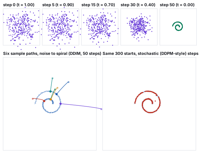
Top: five panels of 300 particles at steps 0, 5, 15, 30 and 50 of DDIM sampling, contracting from a Gaussian cloud into a clean spiral. Bottom left: six colored particle paths from their random starts to their landing points on the spiral. Bottom right: the final positions of 300 particles under stochastic stepping, also on the spiral.
Sampling on the spiral with the exact denoiser. Top: 300 particles at five moments of a 50-step DDIM run. Nothing visible happens for the first fifteen steps because the estimate is the data mean; the shape appears between steps 30 and 50, as the arrows of the score field resolve the arms. Bottom left: six of the paths. Each starts somewhere in the cloud and lands on the spiral, and where it lands depends only on where it started (\(\sigma = 0\)). Bottom right: the same 300 starts with DDPM-style noise at every step land on the spiral too, at different places. Mean distance from a landed particle to the nearest data point: 0.009 for both; a 10-step DDIM run gives 0.064.

4.1 How many steps

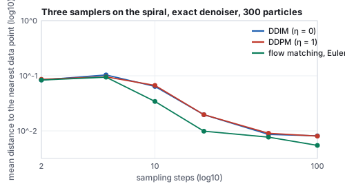
Mean distance from landed particles to the nearest data point against the number of sampling steps, log-log, for DDIM, DDPM and flow matching: all near 0.09 at 2 to 5 steps, DDIM and DDPM together falling to 0.02 at 20 and 0.008 at 50 to 100, flow matching lower from 10 steps on, 0.0055 at 100.
Accuracy against step count on the spiral, 300 particles each, exact denoiser: the mean distance from a landed particle to the nearest data point.
steps25102050100
DDIM (\(\sigma = 0\))0.0840.1030.0640.0200.0090.008
DDPM (\(\sigma\) at its full value)0.0860.0960.0670.0200.0090.008
flow matching, Euler (Section 5)0.0840.0940.0340.0100.0080.006

Below ten steps every sampler lands its particles near the data’s center of mass rather than on the arms (a distance of 0.08 to 0.10 is the width of the spiral’s gaps); from 20 steps the error falls by about a factor of two per doubling, and from 50 it has reached the floor set by the spacing of the 400 data points. Stochastic and deterministic stepping cost the same and land the same; they differ in which point a given start reaches, not in how accurately. Fewer steps trade detail and diversity for speed; distillation trains a student to jump where the teacher walked, down to a handful of steps. Stochastic sampling with many steps is the original DDPM; deterministic sampling with a few dozen is what most systems ship.

4.2 The ODE underneath

The deterministic sampler is not a trick. The forward process is a stochastic differential equation, \(d\mathbf{x} = -\tfrac12\beta(t)\,\mathbf{x}\,dt + \sqrt{\beta(t)}\,d\mathbf{w}\) (the “variance-preserving” SDE), and Anderson’s theorem gives its time reversal as another SDE whose drift involves the score \(\nabla\log p_t\); running it backward with the learned score is DDPM. Every SDE has a companion ordinary differential equation with the same marginal densities at every \(t\), \[ \frac{d\mathbf{x}}{dt} = -\tfrac12\beta(t)\big(\mathbf{x} + \nabla_{\mathbf{x}}\log p_t(\mathbf{x})\big), \] the probability-flow ODE (Song et al. 2021). DDIM is a first-order solver for it, which is why its paths are smooth curves and why a given start always lands at the same place: an ODE has one solution per initial condition. The higher-order solvers that cut the step count (DPM-Solver, Heun’s method in EDM) are the numerical-analysis toolkit of the animation chapter applied to this equation, and the step-count table above is their convergence curve.

5 · Flow matching: the straight-line version

If the goal is an ODE from noise to data, the forward process need not be a diffusion at all. Flow matching (Lipman and others, 2022; rectified flow, Liu and others, 2022) draws the straight line between a data point and a noise point, \[ \mathbf{x}_t = (1 - t)\,\mathbf{x}_0 + t\,\boldsymbol\epsilon, \qquad \frac{d\mathbf{x}_t}{dt} = \boldsymbol\epsilon - \mathbf{x}_0, \] and trains the network to predict that constant velocity from \((\mathbf{x}_t, t)\) by squared error. Sampling is Euler’s method on the learned field from \(t = 1\) down to \(0\). Every ingredient of the diffusion recipe survives (a schedule, in which the weights are now \(1 - t\) and \(t\) rather than \(\sqrt{\bar\alpha}\) and \(\sqrt{1 - \bar\alpha}\); a posterior-mean target; a conditional variant; guidance), and the marginal velocity for a finite dataset is again computable exactly.
The exact marginal velocity With \(\mathbf{x}_t\) Gaussian about \((1 - t)\,\mathbf{x}^{(i)}\) with variance \(t^2\), the posterior over training points has weights \(w_i \propto \exp\big(-\|\mathbf{x}_t - (1 - t)\,\mathbf{x}^{(i)}\|^2/2t^2\big)\), and the expected velocity is \[ \mathbf{v}(\mathbf{x}_t, t) = \mathbb{E}[\boldsymbol\epsilon - \mathbf{x}_0 \mid \mathbf{x}_t] = \frac{\mathbf{x}_t - \hat{\mathbf{x}}_0}{t}, \qquad \hat{\mathbf{x}}_0 = \sum_i w_i\,\mathbf{x}^{(i)}, \] because \(\boldsymbol\epsilon = (\mathbf{x}_t - (1 - t)\mathbf{x}_0)/t\). The velocity points from the current position toward the denoised estimate, scaled by the time left.
Worked example (two points, one Euler step) Data \(\{-1, +1\}\) again, \(t = 0.5\), \(x_t = 0.3\). The scaled points are \((1 - t)\,x^{(i)} = \mp0.5\), the squared distances 0.64 and 0.04, the logits \(-d^2/(2t^2) = -d^2/0.5\): \(-1.28\) and \(-0.08\); the weights \(0.2315\) and \(0.7685\); \(\hat x_0 = -0.2315 + 0.7685 = 0.537\). The velocity is \((0.3 - 0.537)/0.5 = -0.474\). The field is written in forward time; sampling runs it backward, \(x \leftarrow x - \Delta t\,v\), so a negative velocity moves the particle right, toward the \(+1\) point. An Euler step to \(t = 0.4\) gives \(x = 0.3 - 0.1\,(-0.474) = 0.347\); a single jump to \(t = 0\) gives \(x = 0.3 - 0.5\,(-0.474) = 0.537 = \hat x_0\), the current estimate, exactly as a one-step DDIM jump returns \(\hat{\mathbf{x}}_0\). Compare the diffusion denoiser at the same \(x_t\) and a comparable noise level (\(\bar\alpha = \tfrac14\)): \(\hat x_0 = 0.197\). The two processes put different amounts of noise at “\(t = 0.5\)”, so the estimates differ; the mechanism is the same.
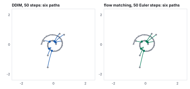
Two panels of the spiral with six particle paths each, from gray starting points to colored landing points: DDIM paths in blue curve toward the data; flow-matching paths in green are nearly straight.
Six particles from the same six starts under DDIM (left) and the exact flow-matching velocity with 50 Euler steps (right). The flow paths are straighter: their length divided by the straight-line distance from start to end is 1.00 to 1.14 for five of the six, against 1.00 to 1.06 for DDIM, with one path in each panel that turns sharply near the data (1.74 and 1.55) because it started between two arms.

Straight paths are the point: an Euler step along a straight line is exact, so a field whose paths are nearly straight can be sampled in few steps, and the table of Section 4 shows flow matching ahead of DDIM at every count from 10 steps on. Rectified flow goes further and re-pairs noise and data along the learned paths to straighten them again (“reflow”), which is how Stable Diffusion 3 and the models after it reach good samples in a few dozen steps and their distilled versions in one to four.

6 · From lookup table to network

Run the exact sampler on the 2,000 digits, each a point of \(\mathbb{R}^{400}\), and every sample lands exactly on a training digit. An exact denoiser for a finite set can only return the set: at the last step the weights are one-hot and \(\hat{\mathbf{x}}_0\) is a member. The demos measure this with the distance from a sample to its nearest training digit (per pixel, in \([-1,1]\) units), and it reads \(0.000\).

Two rows of ten small images. Top row: the exact denoiser's estimate of the clean digit at successive sampling steps, sharpening from a gray blur into a crisp 7 by step 4 and staying there; a pink copy of the nearest training digit, the same 7, at the far right. Bottom row: the same run with the smoothing bandwidth h = 3; the estimate stays a soft blend of strokes to the end and its nearest training digit, a 1, differs from it.
One sample, watched. Each panel is \(\hat{\mathbf{x}}_0\) at steps 0, 2, 4, 6, 8, 10, 13, 16 and 20 of a 20-step run; the tinted panel at the right is the nearest training digit to where the sample landed. Top: the exact denoiser. The estimate is the mean digit at step 0, has chosen a particular 7 by step 4, and lands on it at distance 0.000: memorization. Bottom: the same run with the kernel variance floored (\(h = 3\), below). The estimate stays a smooth average to the end and lands 0.34 per pixel from anything in the set; it is a blend nobody wrote.

The exact denoiser can be made to generalize a little by hand. Add a floor \(h^2\) to the kernel variance, \(1 - \bar\alpha \to 1 - \bar\alpha + h^2\), so that the weights never become one-hot and the average keeps averaging to the end. This is the smooth knob of the digits demo, and it is a kernel density estimator’s bandwidth.
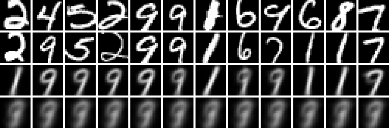
Four rows of twelve digit samples. Row 1 (exact): crisp digits, all copies of training examples. Row 2 (h = 1.5): crisp digits, still copies. Row 3 (h = 3): soft, thick-stroked digits, mostly 9-like and 1-like blends. Row 4 (h = 5): twelve nearly identical blurry blobs.
Twelve samples per row, same twelve starting noises. Bandwidth \(h = 0\): copies of training digits (mean distance to the nearest 0.000). \(h = 1.5\): still copies (0.016). \(h = 3\): novel blends, thick and soft, and mostly of the two most common shapes (0.29). \(h = 5\): every sample is the same blur of the whole dataset (0.43). There is no bandwidth that gives crisp and new digits: a kernel average cannot invent a stroke, only mix strokes. That is the ceiling of any lookup-table denoiser, however smoothed.

A network has no such ceiling, for the reason the networks chapter gave: it is smooth between examples in the space of functions, not of pixels. Trained to approximate the posterior mean on 60,000 digits it never sees the sum; it learns the regularities of strokes that the sum only implicitly contains, and at sampling time it produces images that follow those regularities without being any training image.
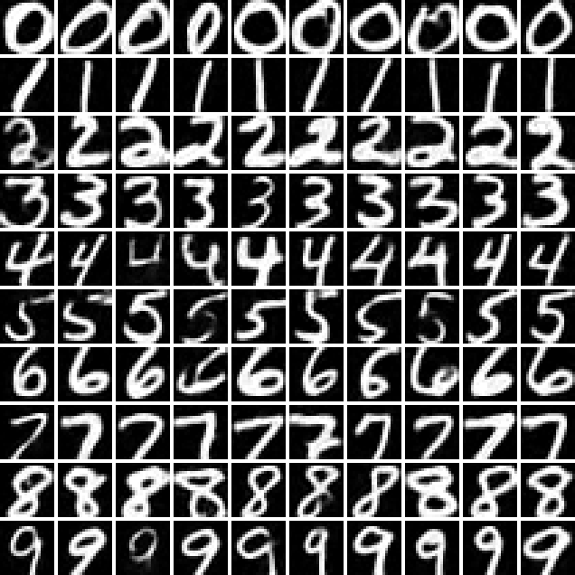

A ten by ten grid of handwritten digits drawn by the trained network, one class per row from 0 to 9, ten different samples each; strokes vary in slant and width within each row.
One hundred digits nobody wrote: the course’s million-weight network, thirty DDIM steps, guidance \(w = 2\), one class per row. Mean distance from a sample to its nearest training digit 0.47 per pixel; the closest of the hundred is 0.18. Nothing here is a copy, and every row is legibly its class.
Two rows of ten images. Top: the sampler's state x_t at ten steps, from pure static to a clean 5. Bottom: the network's estimate of the clean image at the same steps, a soft 5-like blob from the very first step that sharpens into the final 5.
The network drawing a 5, watched. Top row: \(\mathbf{x}_t\) at steps 0, 1, 2, 4, 6, 9, 12, 16, 22 and 30 of a 30-step run (\(t = 1.0, 0.97, 0.93, 0.87, 0.80, 0.70, 0.60, 0.47, 0.27, 0\)). Bottom row: the network’s \(\hat{\mathbf{x}}_0\) at those steps. Already at step 0, given pure static and the label 5, the estimate is a soft average 5; by step 9 the particular slant and loop of this 5 have been decided; the last steps add stroke edges. Compare the exact denoiser’s trajectory above: same schedule, same sampler, but this estimate was never a member of the training set.
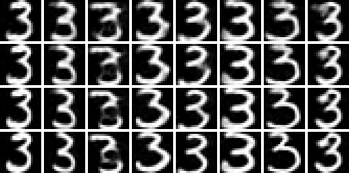
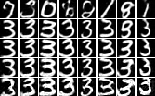
Four rows of eight 3s drawn by the network from the same eight starting noises with 3, 5, 10 and 30 sampling steps: the 3-step row is soft and sometimes malformed, the 5-step row cleaner, the 10- and 30-step rows crisp and nearly identical to each other.
The network with 3, 5, 10 and 30 steps (rows), same eight noises (columns), class 3, \(w = 2\). The mean distance to the nearest training digit is 0.48 to 0.51 per pixel in every row: nearest-neighbor distance does not measure quality, only novelty. What the rows show is that a network trained to predict \(\mathbf{x}_0\) makes a plausible digit in three steps, because its estimate at high noise is already a whole digit rather than a mean; the extra steps decide the details.
See it live Digits nobody wrote (the smooth knob: exact is memorization, \(h\approx3\) makes novel blends, \(h=5\) collapses to one blurry average), then the network draws: the trained denoiser samples digits it never saw, with the class buttons as conditioning and guide as \(w\).
Hands-on The chapter’s spiral and digit figures come from two library files that run in node. From css551/, with node -e "…":
  1. The schedule and the exact denoiser on the spiral:
    import('./lib/core/diffusion.js').then(d=>{
      console.log('abar(0.3)=',d.alphaBar(0.3).toFixed(4),'snr(0.3)=',d.snrDb(0.3).toFixed(2),'dB');
      const sp=d.makeShape('spiral');
      console.log('denoise(0.8,0.6,t=0.5)=',d.denoisePoint(0.8,0.6,0.5,sp).map(v=>v.toFixed(3)));
      for(const st of [5,20,50]) console.log('steps',st,'nearest',
        d.meanNearestDistance(d.sample({data:sp,steps:st,n:300,seed:1}),sp).toFixed(4));});
    Expected: abar(0.3)= 0.7869 snr(0.3)= 5.67 dB, the table’s row; denoise(0.8,0.6,t=0.5)= [ '0.102', '0.158' ], a pull toward the spiral’s center; and steps 5 nearest 0.1034, steps 20 nearest 0.0197, steps 50 nearest 0.0086, the DDIM row of Section 4.
  2. Load the trained network and draw three 7s:
    const fs=require('fs');Promise.all([import('./lib/core/mlp-denoiser.js'),import('./lib/core/diffusion-nd.js')]).then(([md])=>{
      const man=JSON.parse(fs.readFileSync('lib/assets/mnist/mlp-denoiser.json'));
      const w=new Float32Array(fs.readFileSync('lib/assets/mnist/mlp-denoiser.bin').buffer.slice(0));
      const net=md.makeMlpDenoiser(man,w);console.log('weights',net.params,'predicts',net.predicts);
      const out=net.sample({steps:30,m:3,seed:1,cls:7,w:2});
      console.log('ink pixels per sample',out.map(v=>{let k=0;for(const p of v)if(p>0)k++;return k;}));});
    Expected: weights 1002064 predicts x0 and ink pixels per sample [ 94, 90, 58 ]: three 7s of different weights, from three noises. Change cls and seed; print a sample as 20 rows of characters to see it.
  3. In the dots demo, set the steps to 5 and watch the particles stop short of the arms; that is the 0.10 of the table.

7 · Guidance

A conditional denoiser takes the label (or the caption) as an extra input; the network above reads a learned 64-number class vector, the embedding of the networks chapter. Classifier-free guidance (Ho & Salimans 2022) trains the network both with and without its condition \(c\) (the condition is dropped at random, 15 % of the time in the course’s run, and replaced by an eleventh “no class” embedding) and, at sampling time, exaggerates the difference by a scale \(w\):

\[ \hat{\mathbf{x}}_0 \;\leftarrow\; \hat{\mathbf{x}}_0(\varnothing) + w\,\big(\hat{\mathbf{x}}_0(c) - \hat{\mathbf{x}}_0(\varnothing)\big). \]
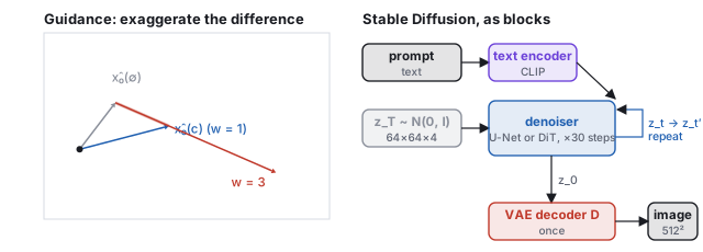
Left: a vector diagram with the unconditional estimate in gray, the conditional estimate in blue, and the guided estimate for w = 3 in red extended along the difference. Right: a block diagram of Stable Diffusion: prompt into a CLIP text encoder, random latent into a denoiser that loops thirty times, then a VAE decoder producing the image once.
Left: guidance is extrapolation. \(w = 1\) is plain conditioning; \(w = 3\) walks three times as far along the direction that distinguishes “a 3” from “any digit”; \(w = 0\) ignores the condition. Right: the block diagram of Section 8.
Worked example (guidance on two numbers) Suppose at some step the unconditional estimate of two pixels is \(\hat{\mathbf{x}}_0(\varnothing) = (0.2, 0.2)\) and the estimate given the class is \(\hat{\mathbf{x}}_0(c) = (0.5, 0.1)\). The class direction is \((0.3, -0.1)\). Then \(w = 1\) gives \((0.5, 0.1)\); \(w = 3\) gives \((0.2, 0.2) + 3\,(0.3, -0.1) = (1.1, -0.1)\), which is then clamped to the valid range \([-1, 1]\); \(w = 0\) gives \((0.2, 0.2)\), the condition ignored. The clamping at large \(w\) is where the saturated, over-contrasted look of heavily guided images comes from.
Five rows of eight digit samples from the same eight starting noises. Row w = 0: an assortment of digits of every class. Rows w = 1, 2, 4: clean 3s of increasing contrast. Row w = 8: 3s with heavy, blotchy strokes and artifacts.
The network asked for a 3 at \(w = 0, 1, 2, 4, 8\) (rows), from the same eight noises (columns). At \(w = 0\) the label is ignored and the noises become whatever digit they were nearest. At \(w = 1\) every column is a 3, each keeping the slant and weight its noise implied. Rising \(w\) makes the 3s more emphatically 3-shaped and then, at 8, over-driven: thick, blotchy, with the clamping visible. Text-to-image systems sit near \(w \approx 7\) on their own scale, past which images saturate and repeat.
Pitfall Guidance is not free, and its cost can be counted. Over eight samples of a 3 at 30 steps, the fraction of pixels saturated at full white (ink) is 7.3 % at \(w = 1\), 8.8 % at \(w = 2\), 10.9 % at \(w = 4\) and 15.9 % at \(w = 8\); the mean pixel value rises from \(-0.42\) to \(-0.25\). Every doubling of \(w\) pushes another few percent of the picture to the rail: strokes thicken, then blot. And a guided estimate is no longer the posterior mean of anything, so the sampler’s accuracy guarantees of Section 4 no longer hold; what it produces is an image that is more of its class than any training image, at the expense of the variety the noise was supposed to supply. The rows of the figure at \(w = 4\) and \(8\) are visibly more alike than the row at \(w = 1\). The remedies in use, guidance intervals that apply \(w\) only in the middle of the run and dynamic thresholding that rescales rather than clips, both aim at the same thing: the class direction without the rail.

8 · From digits to Stable Diffusion: the three scalings

Nothing in the recipe changes between the digit network and the largest image models; three things scale.

the course’s networkStable Diffusion (2022)
the point\(20\times20\) gray, 400 numbersa \(64\times64\times4\) latent (16,384 numbers) standing for a \(512\times512\times3\) image
the conditiona class index, via a learned 64-vectora caption, via CLIP’s text encoder, read at every layer
the networka 3-layer perceptron, \(10^6\) weightsa U-Net (later a transformer), about \(10^9\) weights
the data60,000 digitsbillions of captioned images
the schedule, the loss, the sampler, guidancethe same

The point gets bigger, so diffuse a latent. A \(512\times512\) image is 786,432 numbers; denoising that a thousand times per picture is unaffordable. Latent diffusion runs the whole process on an autoencoder’s \(64\times64\times4\) latent and decodes once at the end (Rombach et al. 2022); that is Stable Diffusion, and it is why the method fits on a gaming GPU. The autoencoder is a variational one (Kingma and Welling, 2014): its encoder outputs a mean and a variance per latent number, the decoder is trained on samples from that Gaussian, and a small penalty keeps the latents near a standard normal, so that the latent space is smooth and every point in it decodes to something. Without that regularization the diffusion model would have to learn a latent distribution full of holes. The decoder is also trained with a perceptual and an adversarial loss, so that fine texture is re-synthesized rather than reproduced; the latent keeps layout, shape and color, and the decoder invents the grain. The condition gets richer, so put text in the class slot. The class embedding the digit network reads becomes a CLIP text embedding consulted at every layer through cross-attention; guidance is unchanged. The network gets bigger. U-Nets in 2020 to 2022, then transformers over image patches (DiT, Peebles & Xie 2023); quality followed scale. The two text-to-image systems that made the public notice in 2022 took different routes to the same place, DALL·E 2 diffusing in CLIP’s embedding space and Imagen conditioning on a large language model’s text embedding.


A Stable Diffusion image of a green, sunlit city street with trees, a tram and people waiting.
Text to image at scale: a Stable Diffusion output for a prompt beginning “utopia at street level in city … solarpunk, green trees”. Prototyperspective · CC0 · via Wikimedia Commons. Same recipe as the digits: a latent of noise, thirty guided denoising steps toward the caption’s embedding, one decode.
Five images of the same prompt and seed at guidance scales 2.5, 7.5, 12.5, 20 and 30; detail and contrast rise, then the image saturates and distorts.
Guidance at scale: one prompt and seed at \(w = 2.5, 7.5, 12.5, 20, 30\). The same arc as the digit rows in Section 7. MrAlanKoh · CC BY-SA 4.0 · via Wikimedia Commons (one row of the original grid).

Two developments matter most to a graphics course. ControlNet (Zhang, Rao & Agrawala 2023) conditions the denoiser on a structural image, a depth map, a normal map or an edge image, and makes it keep that structure while painting the appearance; depth and normals are the pipeline’s own by-products (the viewing chapter, the meshes chapter), so geometry and camera come from the renderer, where you have control, and appearance from the model.
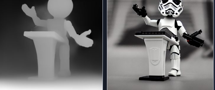
Left: a depth map of a toy robot. Right: a generated image of a stormtrooper lecturing, in the same pose and layout as the depth map.
ControlNet on depth: the depth map on the left fixes the layout, the prompt “Stormtrooper’s lecture” fixes the appearance. A depth buffer is something every renderer in this course already produces. lllyasviel/ControlNet README, depth example · Apache-2.0.

And an image model can train a 3D scene: DreamFusion (Poole et al. 2022) optimizes a NeRF so that its renders, from random viewpoints, score well under a text-conditioned image model, with the gradients flowing back through the differentiable renderer (score distillation; the renderer is the subject of the learned-scenes chapter). Video is the same recipe with a time axis: a block of latents attended across frames (Ho et al. 2022), scaled by 2024 to minute-long clips.

Six frames from a generated clip of a white dragon, evenly spaced in time.
Six of 52 frames of a generated clip. The point being denoised is a block of frames; consistency across the strip is whatever the attention across frames learned, with no scene, camera or physics behind it. Prompted by Lumi’s AI Dreams · public domain · via Wikimedia Commons.

9 · Evaluation: how a generator is judged

A denoiser can be scored by its squared error, but a generator cannot: its samples are supposed to be new, so there is no reference image to compare against, and the metrics of the image-space chapter do not apply. The standard answer compares distributions.

Definition (Fréchet inception distance) Embed a large set of generated images and a large set of real ones with a fixed image network (Inception, at its 2,048-dimensional penultimate layer); fit a Gaussian to each set, with means \(\boldsymbol\mu_g, \boldsymbol\mu_r\) and covariances \(\Sigma_g, \Sigma_r\); report \[ \text{FID} = \|\boldsymbol\mu_g - \boldsymbol\mu_r\|^2 + \mathrm{tr}\big(\Sigma_g + \Sigma_r - 2(\Sigma_g\Sigma_r)^{1/2}\big), \] the distance between the two Gaussians (Heusel and others, 2017). Lower is better; 0 means the two sets have the same first two moments in feature space.
Worked example (a toy FID on the digits) Replace Inception’s 2,048 features by the two principal coordinates of the image-space chapter’s digit cloud, and compare 100 samples against the 2,000 digits. Two halves of the data against each other: 0.12, the noise floor of the estimate. The exact denoiser’s samples (copies of training digits): 0.40. Samples at bandwidth \(h = 5\) (the blurred average): 0.65. The network’s samples: 0.88. Uniform noise: 59.7. The metric separates noise from digits by two orders of magnitude, and it ranks the copies best of all, because copies have exactly the data’s distribution: FID measures whether the samples are distributed like the data, not whether they are new. The blurred average scores better than the network in two dimensions because its mean and spread in the two coarsest coordinates are right and the network’s samples are slightly over-confident (guidance \(w = 2\) narrows the spread); in 2,048 feature dimensions the blur would fail badly, since blur removes exactly the features the network computes.

The real metric has the same two blind spots, at scale. It cannot see memorization: a model that emits training images verbatim scores perfectly. And it depends entirely on the embedding network: features trained on object categories reward object-like texture and are indifferent to global layout, hands, or text, which is why a model can have an excellent FID and draw six fingers. Other metrics fill in: precision and recall on the feature manifold (are the samples on the data’s sheet, and do they cover it), CLIP score for whether a sample matches its caption, and human preference studies, which remain the court of last resort. The course’s own nearest-training-digit distance measures the one thing FID cannot, novelty, and nothing else, as the step-count figure of Section 6 showed.

10 · What still breaks, and what graphics keeps

A diffusion model has no scene, so nothing in it enforces that the cup on frame one is the cup on frame sixty, that objects fall, that hands have five fingers, or that a sign spells a word; it has no camera to move an inch and no edit that leaves everything else fixed. Graphics has exactly those things and lacks the model’s taste for appearance. The field is merging them from both sides: engines that ship generated textures and assets, differentiable renderers that let images train scenes, and world models that generate the next frame in response to a controller input. Neither half erases the pipeline you built; both stand on it.

11 · The papers

YearPaperWhat it added
2014Kingma & Welling, VAEthe variational autoencoder behind latent diffusion
2015Sohl-Dickstein et al.diffusion probabilistic models: destroy, learn to undo
2017Heusel et al.the Fréchet inception distance
2019Song & Ermonthe score (vector field) view
2020Ho, Jain & Abbeel, DDPMpredict the noise; it works at scale
2020Song, Meng & Ermon, DDIMdeterministic, few-step sampling
2021Song et al.diffusion as an SDE; the probability-flow ODE
2021Nichol & Dhariwalthe cosine schedule; learned variances
2021Dhariwal & Nicholguidance; quality past GANs
2022Salimans & Hothe velocity parameterization; progressive distillation
2022Ho & Salimansclassifier-free guidance
2022Rombach et al., latent diffusionStable Diffusion: diffuse in a latent
2022Ramesh et al., DALL·E 2; Saharia et al., Imagentext-to-image at scale, two routes
2022Karras et al., EDMthe design space: schedule, sampler and parameterization untangled
2022Lipman et al., flow matching; Liu et al., rectified flowstraight paths from noise to data
2022Poole et al., DreamFusiontext-to-3D by score distillation
2023Zhang, Rao & Agrawala, ControlNetconditioning on depth, normals, edges
2023Peebles & Xie, DiTthe network is whatever scales

12 · Exercises

Exercise 1 (the exact denoiser) Repeat the worked example of Section 2 with three training scalars \(\{-1, 0, +1\}\), \(\bar\alpha = \tfrac14\), and \(x_t = 0.3\). Which point gets the largest weight, and what is \(\hat x_0\)? Then argue, without computing, what \(\hat x_0\) becomes as \(\bar\alpha \to 0\).
Solution Logits \(-\frac{(x_t - \tfrac12 x^{(i)})^2}{1.5}\): for \(-1, 0, +1\) they are \(-0.4267, -0.0600, -0.0267\). Softmax weights \(0.254, 0.367, 0.379\); the \(+1\) point wins narrowly over \(0\). \(\hat x_0 = -0.254 + 0 + 0.379 = 0.125\). As \(\bar\alpha \to 0\) the logits all tend to \(-x_t^2/2\), the weights become equal, and \(\hat x_0\) tends to the data mean, \(0\).
Exercise 2 (the schedules) At what \(t\) does the linear-\(\beta\) schedule reach the signal-to-noise ratio the cosine schedule has at \(t = 0.5\), and what fraction of its steps does it spend below that level?
Solution The cosine schedule is at 0 dB at \(t = 0.5\); the linear table reads \(-1.8\) dB at \(t = 0.3\) and \(+2.9\) dB at 0.2, so it crosses 0 dB near \(t = 0.27\). It then spends about 73 % of its steps on images that are more noise than signal, against 50 % for the cosine schedule; the network trained on it sees the near-clean regime, where stroke edges are decided, in fewer than a third of its training examples.
Exercise 3 (parameterizations) From the worked point of Section 2.1, recover \(\hat{\boldsymbol\epsilon}\) from \(\hat{\mathbf{v}}\) with \(\hat{\boldsymbol\epsilon} = \sqrt{1-\bar\alpha}\,\mathbf{x}_t + \sqrt{\bar\alpha}\,\hat{\mathbf{v}}\), and check the first coordinate.
Solution \(0.8922\times0.8662 + 0.4517\times0.3974 = 0.7728 + 0.1795 = 0.9523\), the worked \(\hat\epsilon_1\). The pair \((\hat{\mathbf{x}}_0, \hat{\boldsymbol\epsilon})\) and the pair \((\mathbf{x}_t, \hat{\mathbf{v}})\) are related by a rotation by the angle whose cosine is \(\sqrt{\bar\alpha}\), which is where the name “velocity” comes from: \(\mathbf{v}\) is the derivative of \(\mathbf{x}_t\) with respect to that angle.
Exercise 4 (a step of the sampler) Using the numbers of the Section 4 example, compute where the particle would go if the next time were \(t' = 0\) (a single jump to the end) instead of \(0.6793\).
Solution At \(t' = 0\), \(\bar\alpha = 1\), so the noise weight is \(\sqrt{1 - 1} = 0\) and \(\mathbf{x}_0 = 1\cdot\hat{\mathbf{x}}_0 = (0.0367, 0.1490)\): the sampler would output the current estimate, which at this noise level is a point near the middle of the spiral, not on it. That is what a one-step sampler does: it returns the blurred mean. Many small steps let the estimate sharpen as the noise falls.
Exercise 5 (flow matching) Repeat the flow-matching example at \(t = 0.9\), \(x_t = 0.3\). Compare the velocity with the one at \(t = 0.5\).
Solution Scaled points \(\mp0.1\); distances \(0.16\) and \(0.04\); logits \(-d^2/(2\cdot0.81)\): \(-0.099\) and \(-0.025\); weights \(0.482\) and \(0.518\); \(\hat x_0 = 0.037\); velocity \((0.3 - 0.037)/0.9 = +0.292\), so the backward step moves the particle left, toward the origin: \(x = 0.3 - 0.1(0.292) = 0.271\). At high noise the estimate is nearly the data mean and the field mostly shrinks the cloud toward it; at \(t = 0.5\) the same particle had committed to the \(+1\) side and the velocity had changed sign. A flow path first contracts, then chooses.
Exercise 6 (PSNR) The table in Section 1 gives the PSNR of the noised digit at \(t = 0.5\) as 8.5 dB. Using PSNR \(= 10\log_{10}(1/\text{MSE})\) on the \([0,1]\) scale, what mean squared error is that, and roughly how large is the typical per-pixel error?
Solution \(\text{MSE} = 10^{-0.85} = 0.14\), a root-mean-square error of 0.37 on a scale where black is 0 and white is 1: more than a third of the full range per pixel, and the 7 is still readable. Legibility lives in the coarse structure, which is why the exact denoiser and the network both recover the coarse structure first.
Exercise 7 (guidance) With \(\hat{\mathbf{x}}_0(\varnothing) = (0.2, 0.2)\) and \(\hat{\mathbf{x}}_0(c) = (0.5, 0.1)\), what \(w\) first pushes a coordinate outside \([-1, 1]\)? What does the picture look like when many coordinates are clamped?
Solution The first coordinate is \(0.2 + 0.3\,w\), which exceeds 1 at \(w > 2.67\); the second, \(0.2 - 0.1\,w\), reaches \(-1\) only at \(w = 12\). Clamping many coordinates flattens them to pure black or white: saturated, high-contrast, posterized images, the \(w = 8\) row of Section 7 and the right end of the guidance strip in Section 8.
Exercise 8 (why a latent) Stable Diffusion’s latent is \(64\times64\times4\) for a \(512\times512\times3\) image. By what factor is the denoiser’s input smaller, and what work did the autoencoder do to make that possible?
Solution \(786{,}432 / 16{,}384 = 48\). The autoencoder learned which 16,384 numbers suffice to redraw a plausible photograph: it discarded sensor noise and fine texture that a decoder can re-synthesize, and kept layout, shapes, and colors. The diffusion model then only has to learn the distribution of those, which is a far easier sheet to learn than the one in pixel space.
Exercise 9 (the network, with code) Using the hands-on snippet, sample eight 3s at 30 steps with \(w = 1\) and with \(w = 8\), and count the pixels at exactly \(+1\) in each set. Which set has more, and by how much?
Solution The generator’s run gives 7.3 % of pixels at \(+1\) for \(w = 1\) and 15.9 % for \(w = 8\), about twice as many; a run with another seed moves the numbers by a percent or two. The extra white is the clamped extrapolation of Section 7 made countable: guidance thickens strokes until they saturate.
Exercise 10 (evaluation) A model that has memorized its training set and a model that draws perfect new images of the same distribution get the same FID. What second measurement separates them, and what does it cost?
Solution The nearest-training-neighbor distance of Section 6: near zero for the memorizer, comparable to the data’s own nearest-neighbor spacing for the honest model. Its cost is a search over the whole training set per sample, which for a billion-image set is done approximately with the embeddings of the networks chapter and a nearest-neighbor index, and it is exactly the audit that copyright disputes over generated images turn on.